Lecture 1: Introduction to Neural Networks
Goals of neural networks
The goal of this course is to learn to build neural neural networks, but first we should make sure that we understand what neural networks do and why we’d be interested in learning about them in the first place. You’re probably already familar with a lot of the real-world applications of neural networks, as in the past few years they’ve changed the way we use technology. Systems for everything from voice recognition, to photo-editing, to text and image generation and more now are largely built on the foundation of neural networks. Let’s start by introducing a few broad categories of neural network applications along with some specific examples that you may or may not have seen.
Prediction
In prediction applications neural networks are used to assign a label or a prediction to a given input. Examples of applications using neural networks for prediction include:
Image classification (Example: Google Lens)
Image classification applications like Google Lens can take an image as input and identify the contents of the image using neural networks. This task will be the focus of one of the later modules in the course.

Credit: Google
Medical diagnosis
Does a patient have lung cancer? Neural networks for medical diagnosis might be able take in a patient s symtoms and test results and give an answer.

Credit: Microsoft Research
Detection
In detection applications, neural networks are used to identify any instances of a particular pattern in a given input. For example:
Voice recognition (Example: Siri)
When you say “Hey Siri!” and your phone responds, it was a neural network that recognized your voice; taking as input the audio captured by your phone’s microphone and detecting any instances of the activation phrase.

Credit: Apple
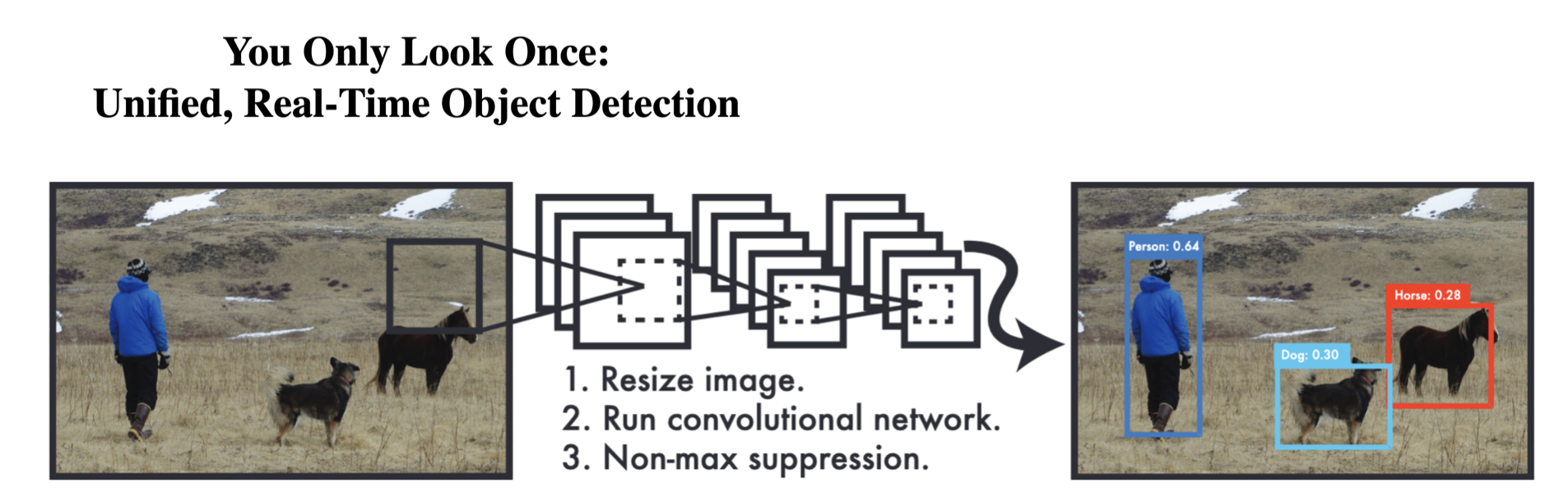
Object detection (Example: YOLO)
Object detection neural networks like YOLO (You Only Look Once) can identify multiple objects in an image. These types of networks are often used in applications like autonomous cars, which need to identify vehicles, pedestrians and other hazards on the road.
Generation
Possibly the most widely discussed application of neural networks in recent years has been generative models, that is models that can generate realistic new data such as images and text.
Text generation (Example: ChatGPT) Large language models, such as the GPT models that power ChatGPT, use neural networks to synthesize realistic language.

Credit: OpenAI
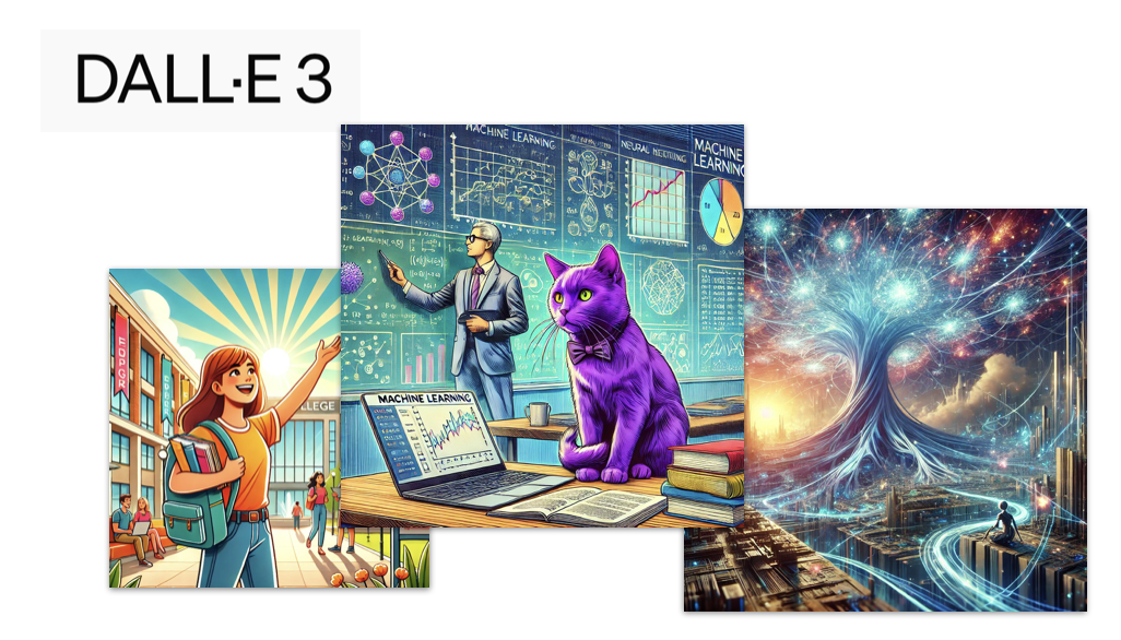
Image generation (Example: Dall-E 3) Deep generative models for images similarly can generate realistic images.
Transformation
Transformation tasks take existing data in the form of images or text and create new and improved versions.
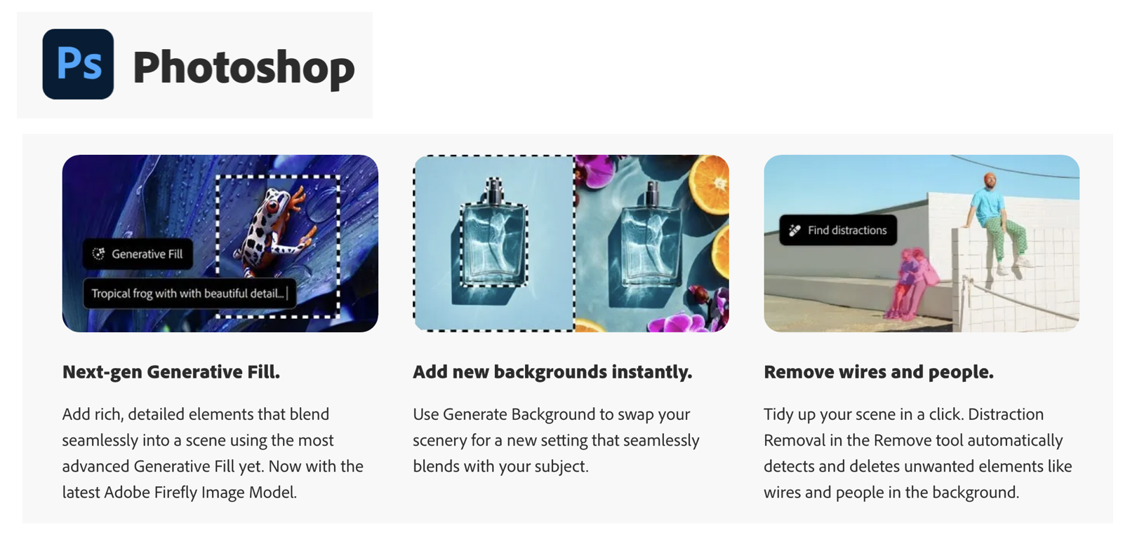
Photo editing (Example: Adobe Photoshop)
Image editing tools like Photoshop use neural networks to output enhanced versions of images, either adjusting properties like color or even filling in missing parts of images!
Credit: Adobe
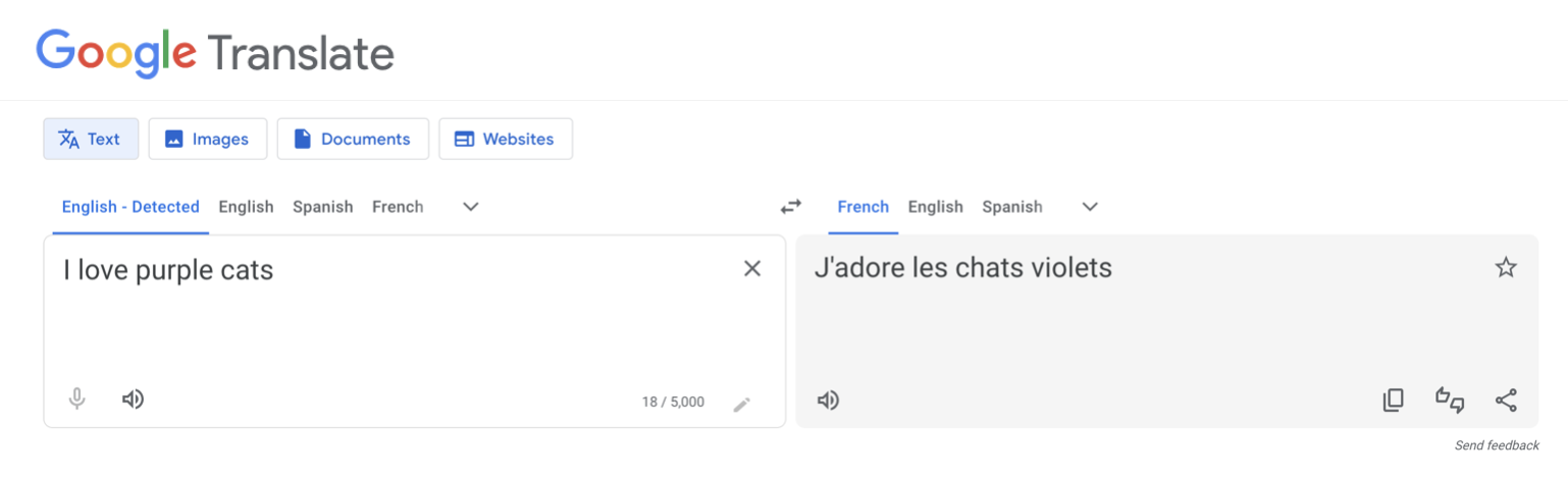
Photo editing (Example: Google Translate)
Translation tools like Google translate use neural networks to map text in one language to another much more effectively than prior methods.
Credit: Google
Approximation
Molecular dynamics (Example: AlphaFold)
Neural networks are finding applications in the physical sciences allowing researchers to create approximate simulations of complex physical systems such as molecules. AlphaFold uses neural networks to predict the structure of proteins given their chemical composition.
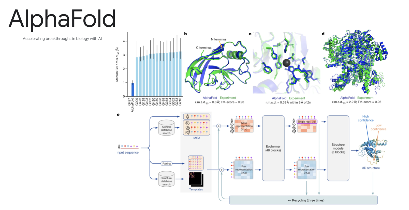
Credit: Google
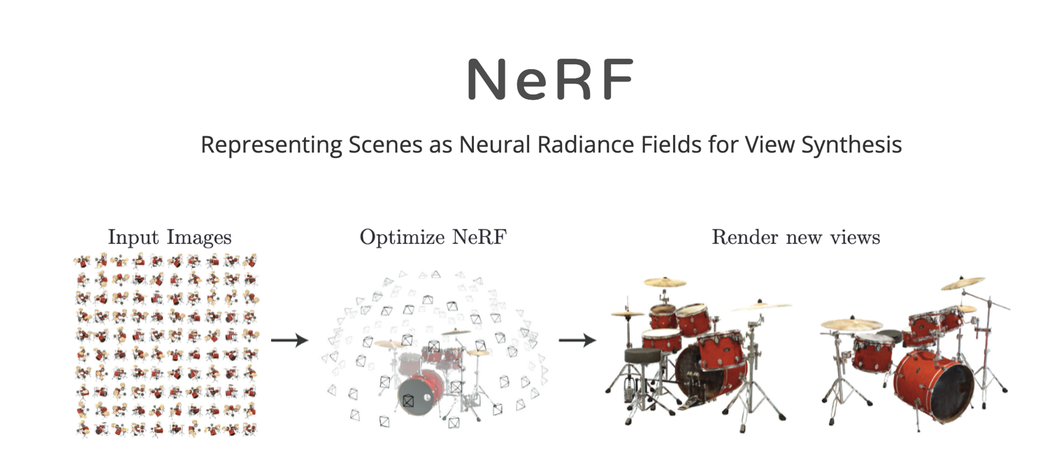
Rendering (Example: NeRFs)
Neural radiance fields (or NeRFs for short) use neural networks to quickly approximate new views of a 3d scene without the need for traditional modeling and rendering.
Prediction problems
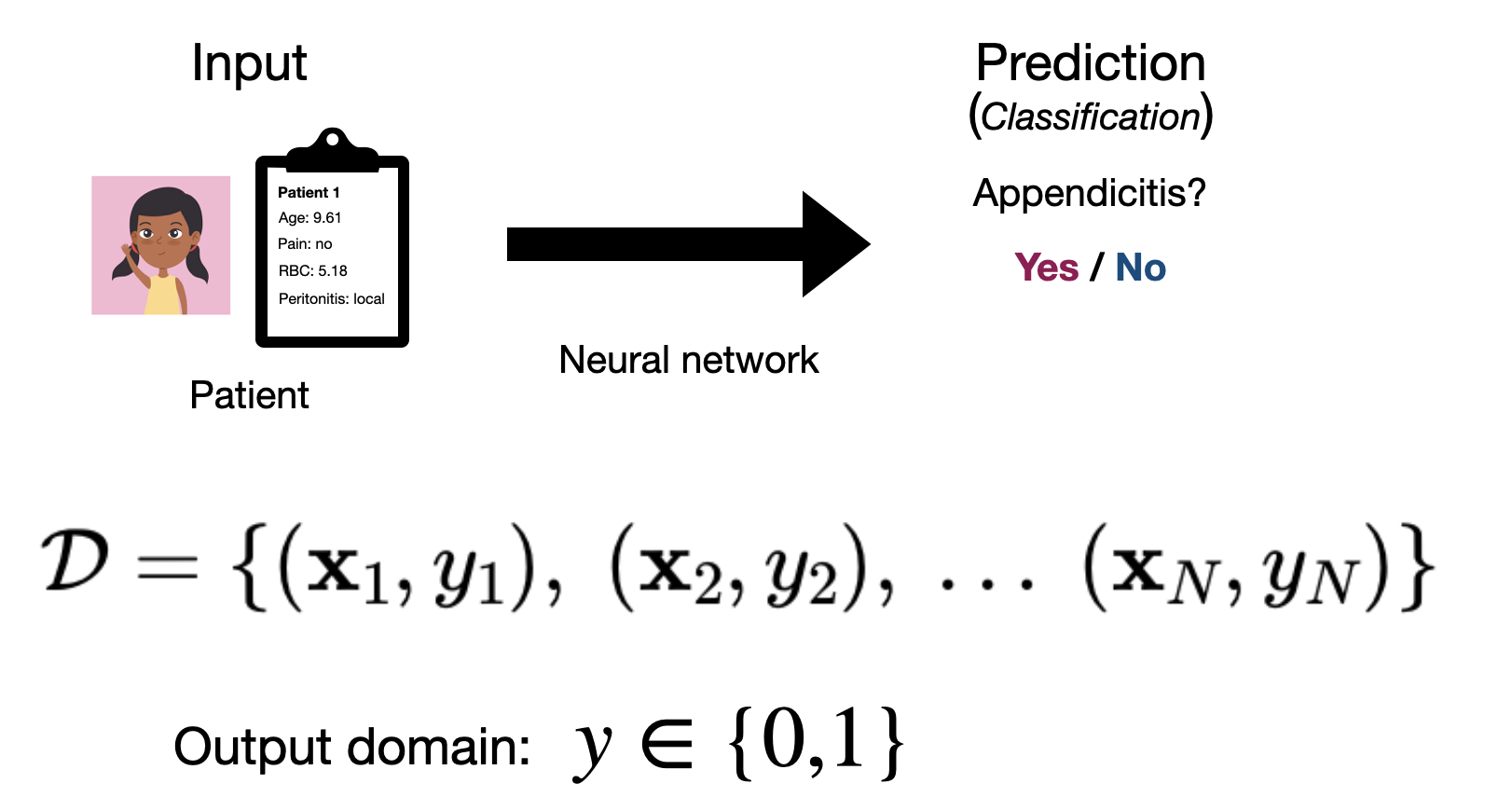
We’ll cover most of these application categories in the course, but we’ll start our journey with what is likely the most common, prediction problems. As a motivating example, we’ll put ourselves in the shoes of a medical professional. In this context, we will likely want to be able to predict if a given patient has a disease, such as appendicitis. So we want a system that can take in some information about our patient and use it to make an informed prediction as to whether or not our patient has a given condition.
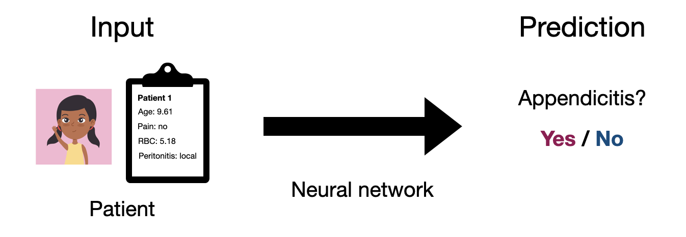
Let’s introduce some notation, so that we can start to formalize this problem a bit better. We’ll use \(\mathbf{x}\) to denote the input to our system, which we’ll call an observation. In this case our observation is a collection of information we have about our patient, e.g. age, prior conditions, test results, etc. Likewise, we’ll use \(y\) to denote the output of our system, which we’ll call a label. In this case our label is a determination of whether or not our patient has the condition. So ultimately what we want is a mapping from any input \(\mathbf{x}\) to an output \(y\). Mathamatically, what we want is a function.
\[ \text{Input: } \mathbf{x} \underset{predict}{\longrightarrow} \text{ Output: }y, \quad y=f(\mathbf{x}) \]
Ultimately, what most of this class is about is simply how to find a function \(f\) that does a good job of making these sorts of predictions in the real world. That may sound simple enough, but it practice it can be very difficult! Neural networks are a class of functions that are very powerful for a wide variety of problems.
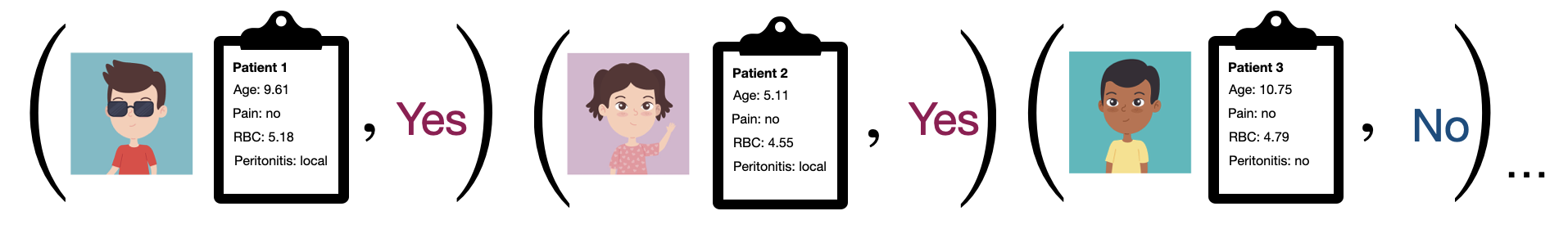
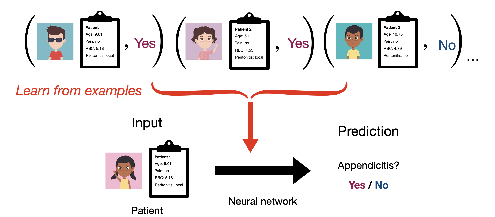
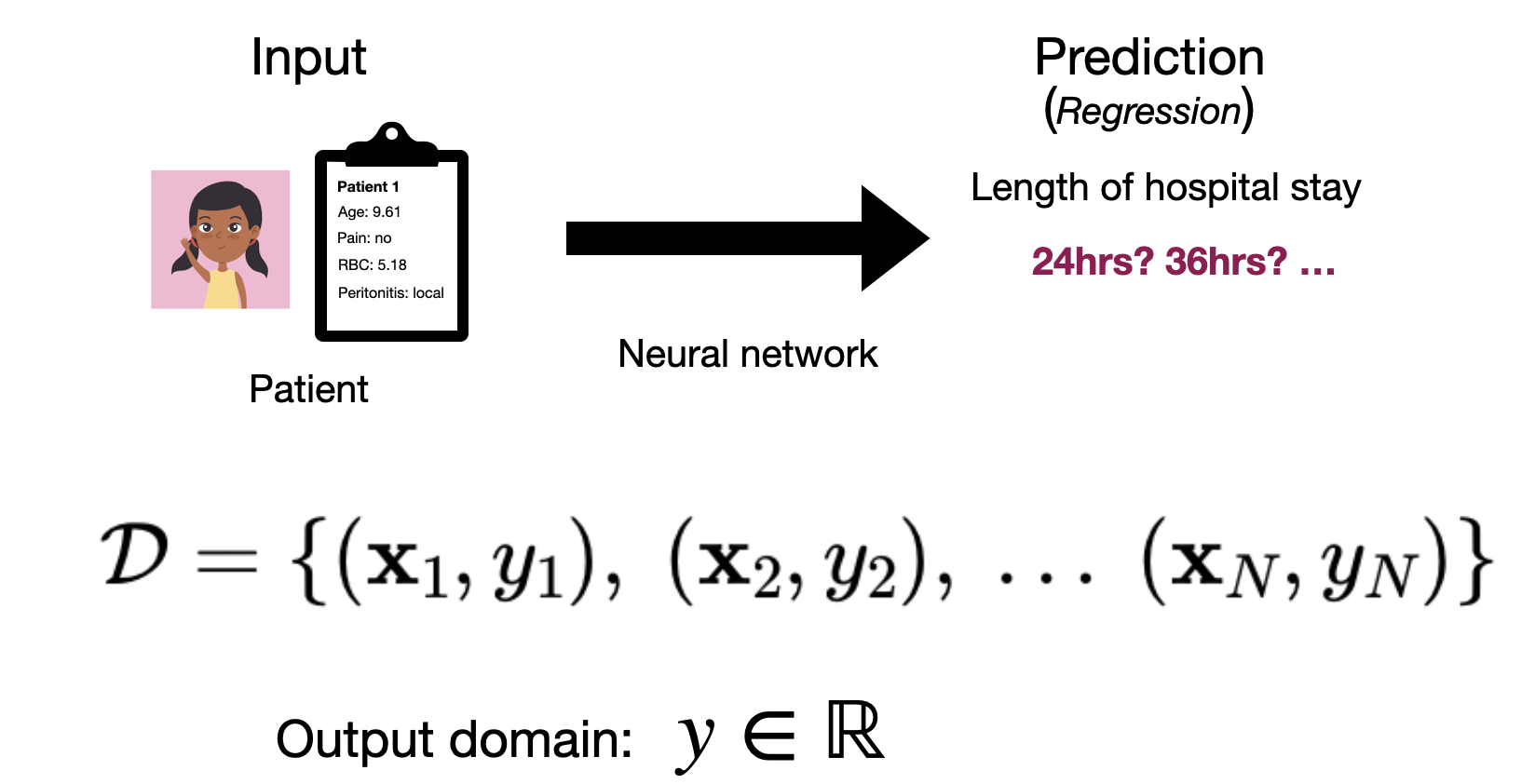
As a preview of what’s to come, our general approach will be to start with a dataset \(\mathcal{D}\) made up of \(N\) pairs of inputs ( \(\mathbf{x}\) ) and outputs ( \(y\) ):
\[ \mathcal{D} = \{ (\mathbf{x}_1, y_1),\ (\mathbf{x}_2, y_2),\ ...\ (\mathbf{x}_N, y_N)\} \]
We’ll then try to choose a function \(f\) that does a good job matching the mapping expressed by this dataset. The fact that we typically learn neural network functions from examples is why we generally consider neural networks to be part of the field of machine learning. We’ll get back to how this process works later. For now, let’s focus on what our data actually looks like in practice.
Types of data
The first step in all of this is going be thinking about how to translate a real-world input like a patient, image, text record etc. as a mathamatical object \(\mathbf{x}\) that we can reason about abstractly and ultimately represent in a computer program. We’ll do the same for our output \(y\) in a moment.
Tabluar data
If you’ve worked with Excel, SQL or even many physical records, you’re likely familiar with the concept of tabular data. Tabular data essentially refers to any data that we can easily represent in a table format. As this could mean a few different things, when we talk about tabular data in this class, we’ll specifically be refering to data in what is often called the tidy data format.
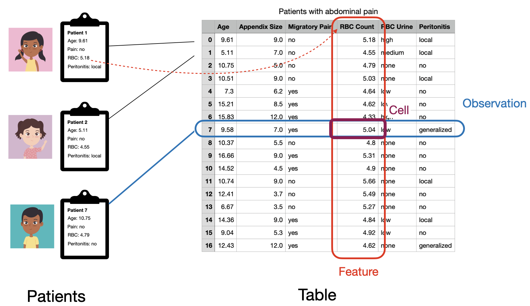
Tidy data
We’ll say that data is in in the “tidy” format if each observation is represented with a single row of our table and each feature is represented with a single column. An observation is an entity, such as a patient in a hospital, that we may want to make preditions about. A feature (or variable) represents some measureable property that every observation has. For the patients in our example the set of features might correspond to measurements like the heart rate, blood pressure or oxygen level of each patient, as well as properties like the patient’s name, age and gender. This organizaton makes it easy to find any given measurement for any given patient (just use the row and column coordinates in the table). For tabular data we’ll assume that the ordering of both rows and columns in our table has no special significance, so could change the ordering of either without altering what our table represents.
Note that how we organize a set of measurements into observations and features isn’t nessecarily fixed, and might change depending on our goals. For example, if our goal is to predict whether a patient has some given underlying condition, we might have one observation per patient. Alternatively, if a given patient visits the hospital several times and our goal is to predict whether a patient will be admitted overnight for a given visit, we might have one observation per visit.
Variable types
The idea of tidy data should also be intuitive to programmers familiar with the object-oriented programming paradigm. There we organize our data in objects (observations) where each object has a common set of properies (features). Just as in object oriented programming, its important to consider the type of each feature, which defines what values it can take and what operations we can perform on it. We’ll consider a few useful general feature types and how we might map them to concrete types in code.
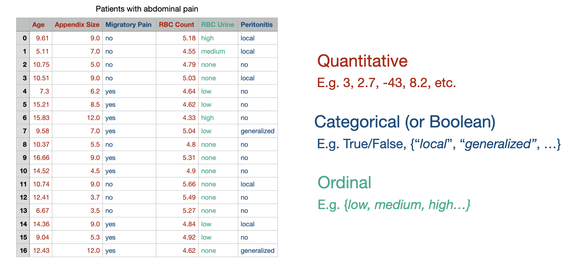
Quantitative features
Quantitative features are simply numbers like our patient’s blood pressure, heart rate etc. We can further subdivide this category into integer features, that we’d encode as integer types (e.g. int, uint) and real-valued features that we’d encode as floating point values (e.g. float).
Categorical features
Categorical features are features that can only take a few distinct, non-numerical values. For example this could be the department that a patient was admitted to ({ER, Neurology, Obstetrics, Dermatology, etc.}) or the patient’s gender identity ({female, male, non-binary, etc.}). These values might be best encoded through an enum type, but are typically encoded as either a string or int in practice.
Boolean features are a special case of categorical features with only two possible values. They could be encoded as an bool or int type.
Ordinal features
Ordinal features are something of a middle-ground between quantitative and categorical features. They represent features where the possible values have a well-definded ordering (like numbers), but no concept of distance (like categorical values). For example our patients might be assigned a priority level that takes the values low, medium or high. In this case it’s well-defined to say that low < medium < high, but asking for the result of high - low is not defined. We might encode these features as int types as well.
General “nomial” features
Non-numerical features that don’t have a fixed set of possible values is what we’d call nominal or unstructured data. While it’s common in many contexts to see such values within tabluar data, for neural networks we’ll generally treat them as their own data type, outside of the tidy, tablular data paradigm.
Matrix data
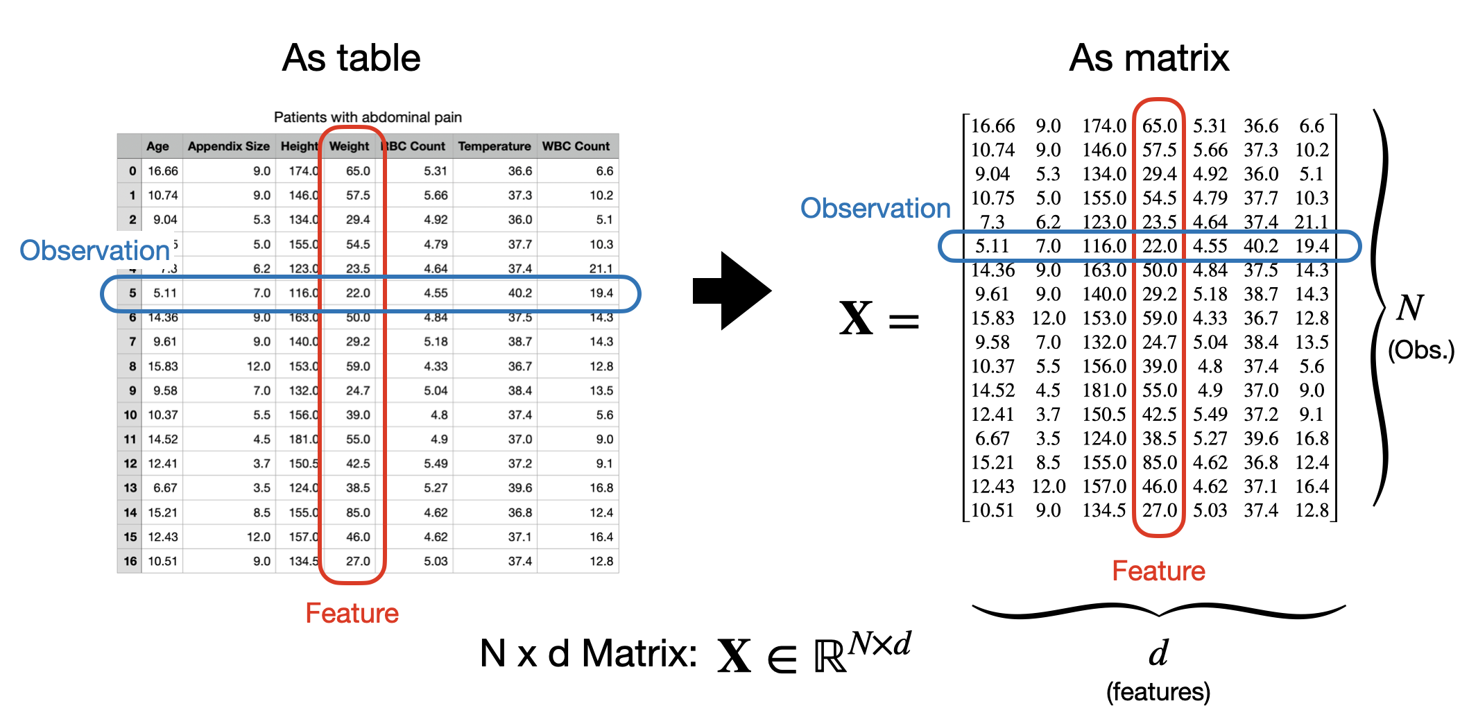
While tables are useful for reading and understanding datasets, as we’ve seen, we want to think about neural networks as mathamatical functions of our data. Therefore, in order to work with them we’ll usually need to abstract away from the specifics of our data into a more convenient mathamatical form. In particular, as tablular data has 2 dimensions (observation rows and feature columns), the natural way to think about a dataset mathamatically is as a matrix. By convention, we’ll usually think about our data as an \(N \times d\) matrix, where we have \(N\) observations and \(d\) features and we’ll typically call this matrix \(\mathbf{X}\).
Under this convention, the first index into our matrix will denote the row or observation and the second, the column or feature. In code, we’ll use numpy arrays to represent matrices, which work similarly.
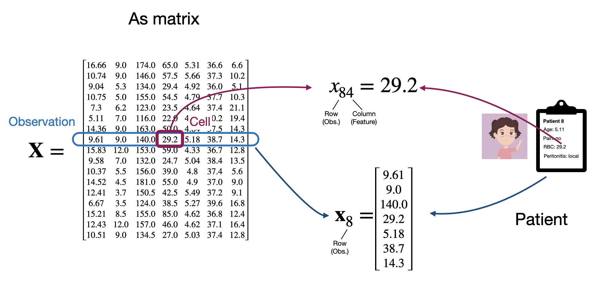
We can also think about each row as being a vector of length \(d\) representing a single observation. So we’ll say that each observation \(\mathbf{x}_i\) is a \(d\)-dimension vector \(\mathbf{x}_i \in \mathbb{R}^d\). This is why so far we’ve used the bold (\(\mathbf{x}\)) notation.
Here it’s worth pointing out a bit of a notational quirk that can get a little confusing. A vector is a 1-dimensional object; we can think of it as a 1-d array in code. However, when we do mathamatical operations involving both matrices and vectors, it’s often convenient to treat a vector as either a \(d \times 1\) matrix, also known as a column vector, or as a \(1 \times d\) matrix (row vector).
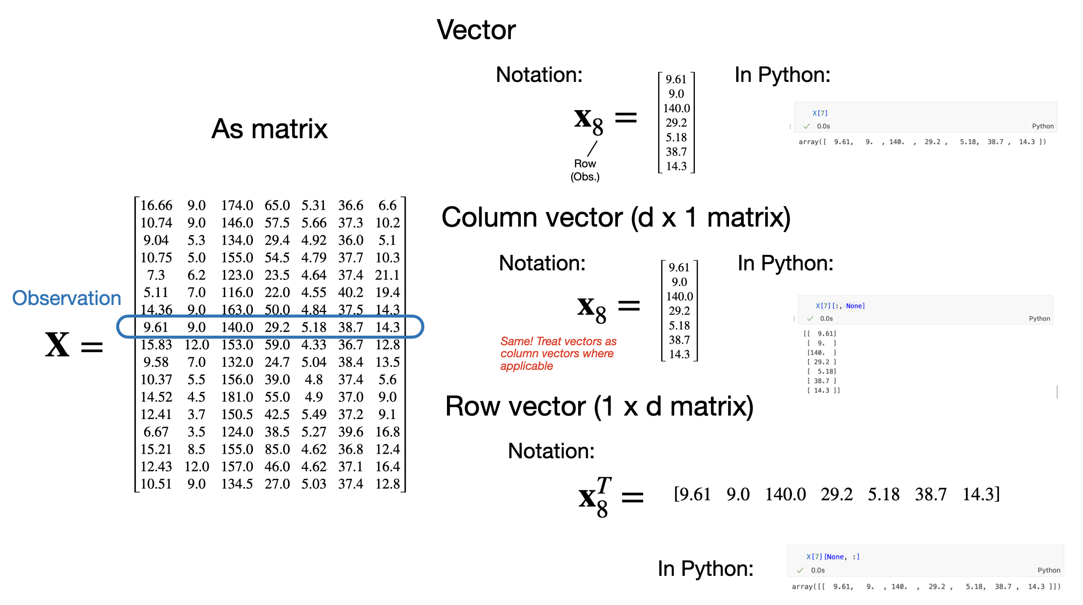
By convention, in mathamatical expressions we’ll assume that by default, any vector we refer to will be treated as a column vector, even if the vector was a row in a matrix. If we want to treat a vector as a row vector, we will explicitly transpose it. This can get confusing so it’s worth keeping this in your head as we move forward. Under this convention, we might think about our matrix of all observations as:
\[\mathbf{X} = \begin{bmatrix} \mathbf{x}_1^T \\ \mathbf{x}_2^T \\ \mathbf{x}_3^T \\ \vdots \end{bmatrix} = \begin{bmatrix} x_{11} & x_{12} & x_{13} & \dots \\ x_{21} & x_{22} & x_{23} & \dots \\ x_{31} & x_{32} & x_{33} & \dots\\ \vdots & \vdots & \vdots & \ddots \end{bmatrix}\]
This will become relevant when reading mathematical expressions of matrices and vectors in this class. For example, consider the two vectors \(\mathbf{a}\) and \(\mathbf{b}\).
\[ \mathbf{a} = \begin{bmatrix} 2 \\ 1 \\ 3\\ \end{bmatrix},\\ \mathbf{b} = \begin{bmatrix} 1 \\ 4 \\ 2\\ \end{bmatrix}, \\ \]
We can write the dot product as:
\[ \mathbf{a}^T \mathbf{b} = \big{[} 2 \ \ \ 1 \ \ \ \ 3 \big{]} \begin{matrix} \begin{bmatrix} 1 \\ 4 \\ 2\\ \end{bmatrix} \\ \\ \\ \end{matrix} =12 \]
Similarly we can write an outer product as:
\[ \mathbf{a} \mathbf{b}^T = \begin{matrix} \begin{bmatrix} 2 \\ 1 \\ 3\\ \end{bmatrix} \\ \\ \\ \end{matrix} \big{[} 1 \ \ \ 4 \ \ \ \ 2 \big{]} = \begin{matrix} \begin{bmatrix} 2 & 8 & 4 \\ 1 & 4 & 2 \\ 3 & 12 & 6 \end{bmatrix}\\ \\ \\ \end{matrix} \]
Encoding non-quantitative features
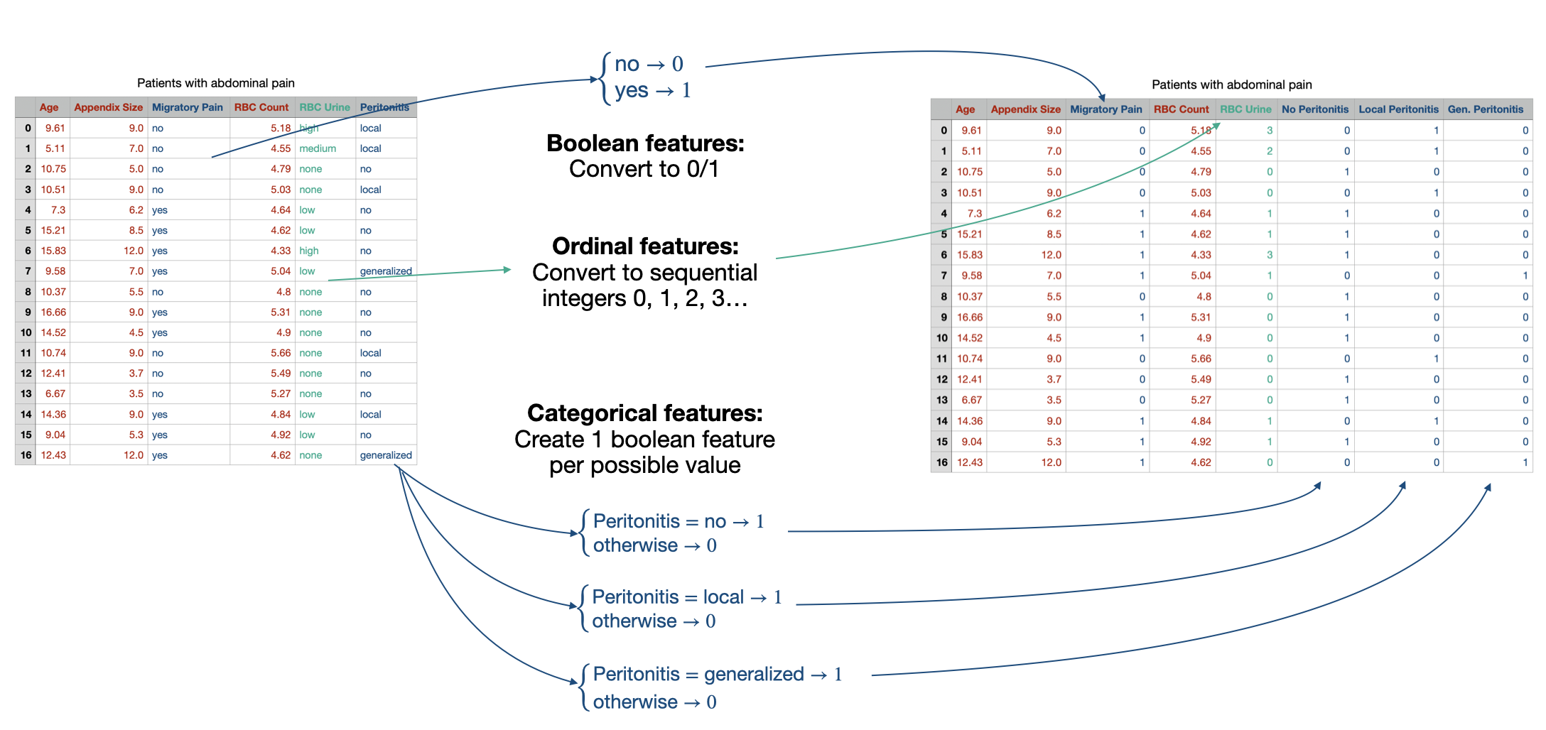
You might be wondering at this point: if we’re treating everything as matrices and vectors, how do deal with features that aren’t inherently real-valued numbers? Generally the approach will be to convert them into real numbers in some way.
Integer features are straightforward; we can easily treat them as real numbers already and in code we can simply cast them. We’ll typically map ordinal features to the first few non-negative integers, e.g. \(\{\text{none},\ \text{low},\ \text{medium},\ \text{high} \} \rightarrow \{ 0, \ 1, \ 2, \ 3 \}\). Boolean features are usually mapped to either \(\{0, 1\}\) or to \(\{-1, 1\}\). Finally categorical values are typically first mapped to a set of boolean values. If a categorical feature as \(c\) possible values, then it will be mapped to \(c\) new boolean variables, each indicating whether the original feature had that value. This is often called one-hot encoding.
We’ll talk (a lot) about unstructured text later in this course, so for now will just worry about categorical/ordinal features.
Label types
For our discussion of prediction problems, we’ll assume that the label that we want to predict is just a single value, which is why we’ve used the scalar notation \(y\).
If our labels are real numbers \(y \in \mathbb{R}\), e.g. if we’re trying to predict the number of hours a patient will stay in the hospital, then we’ll say that we have a regression problem.
Alternatively, if our labels are categorical values, e.g. we’re trying to predict whether or not a patient has appendicitis, \(y \in \{\textit{healthy}, \textit{appendicitis}\}\), then we’ll say that we have a classification problem.
If we have a full dataset of \(N\) observations and labels, we could refer to the collection of \(N\) labels as a vector \(\mathbf{y} \in \mathbb{R}^N\).
Other types of data
We’ll focus on tabular data for the first part of this course, but it’s far from the only type of data that we’ll consider. We won’t go into detail here about representing these types of data, we’ll leave that until we introduce the relevant neural network material.
Image and field data
Images are one of the most common inputs to neural networks for many real-world problems. A single image typically consists of thousands to millions of individual measurements making up the pixels of the image (each “pixel” represents the color or brightness of the image at a given location). In tabular data we generally assume each feature has a different interpretation and the order of the features isn’t inherently meaningful. In image data, our features all have the same interpretation (as pixels), and a specific configuration as a 2-dimensional grid.
More generally, we can think of image data as being a member of the larger category of field data. Field data refers to data where every point in a given space has a value or set of values associated with it. This includes image data (each pixel has a brightness or red, green and blue color values), as well as things like video (with a third, time dimension), audio (with only a time dimension), 3-d medical scans (with x, y and z spatial dimensions) and climate data (latitude and longitude coordinates) among others.
Text and sequence data
Text is another widely used application of neural networks. In this case our observation could be a sentence or paragraph of text. More generally, we can frame this as a variable-length sequence of categorical features (or tokens). Beyond text, we can also frame things like genetic data in this way.
Graph/network data
In many cases our data might be defined not just by the features of each observation, but also by the relationships between observations. In this case we have what we’d call graph or network data. A classic example would be social networks, where the relationships between people (e.g. whether or not they are friends) is of upmost importance. Other examples include things like protein structures, where the configuration of atoms in a molecule is as important as the types of the atoms.
Multi-modal data
In many cases it’s also common to consider more than one type of data at once. For example, a diagnosis system might take in an x-ray image, text of doctor notes and tabular test result data as inputs to its prediction function. We this multi-modal data, as it has multiple different types or modes in one (image, text and tabluar).