Prerequisites for neural networks

Linear algebra prerequisites

We will begin with a review of many of the basic concepts from linear algebra that we will need for this course. As we go through these concepts we will see how to implement them in Python.

Numpy

Numpy Is the linear algebra library that we will be using for much of this class (later on we will introduce PyTorch, which is more geared towards neural networks). The standard way to import Numpy is:

import numpy as np

The most basic object from Numpy that we will just is the array (np.array), which will represent vectors matrices and even higher-dimensional objects known as tensors.

Scalars

Scalars are just single numbers. In our math we will typically denote scalars with a lower-case letter. For example, we might call a scalar \(x\) and give it a value as \(x=3.5\). In code this would be written as:

x = 3.5

# or as a 0-dimensional numpy array
x = np.array(3.5)

In general, we will assume that scalars are real numbers meaning decimal numbers in the range \((-\infty, \infty)\). We can denote this as \(x \in \mathbb{R}\), meaning “\(x\) is in the set of real numbers”.

Vectors

Vectors are ordered lists of numbers, as shown below. We will typically denote vectors with bold lower case letters, such as \(\mathbf{x}\).

\[ \mathbf{x} = \begin{bmatrix} 2\\ 5\\ 1\end{bmatrix} \]

This bold notation is common, but not universal, so expect that external resources may denote things differently!

In Numpy, we can create an array object representing a vector by passing np.array a list of numbers.

x = np.array([2, 5, 1])

Other useful vector creation functions

Constants:

a = np.zeros(5) # Create a size 5 vector filled with zeros
print(a)
a = np.ones(5) # Create a size 5 vector filled with ones
print(a)

[0. 0. 0. 0. 0.]
[1. 1. 1. 1. 1.]

Integer ranges:

a = np.array([1,2,3,4,5,6,7])
print(a)
# or equivalently, using Python iterables:
a = np.array( range(1,8) )
print(a)
# or the NumPy function np.arange:
a = np.arange(1, 8)
print(a)

[1 2 3 4 5 6 7]
[1 2 3 4 5 6 7]
[1 2 3 4 5 6 7]

Decimal ranges:

b = np.linspace(1.0, 7.0, 4) # length-4 vector interpolating between 1.0 and 7.0
print(b)
c = np.logspace(0.0, 2.0, 5) # length-7 vector interpolating between 10^0 and 10^2 logarithmically
print(c)

[1. 3. 5. 7.]
[  1.           3.16227766  10.          31.6227766  100.        ]

Combining vectors

a = np.concatenate([b, c]) # length 4 + 7 vector with the elements of both b and c

The individual numbers in the vector are called the entries and we will refer to them individually as subscripted scalars: \(x_1, x_2,…,x_n\), where \(n\) is the number of entries or size of the vector.

\[ \mathbf{x} = \begin{bmatrix} x_1\\ x_2\\ x_3\end{bmatrix} \]

We may say that \(\mathbf{x} \in \mathbb{R}^n\) to mean that \(\mathbf{x}\) is in the set of vectors with \(n\) real-valued entries. In numpy we can access individual elements of a vector using [] operators (note that numpy is 0-indexed!).

x[0]

np.int64(2)

A vector represents either a location or a change in location in \(n\) -dimensional space. For instance, the \(\mathbf{x}\) vector we defined could represent the point with coordinates \((2, 5, 1)\) in 3-D space or a movement of 2 along the first axis, 5 along the second axis and 1 along the third axis.

Manim Community v0.18.1

Vectors as data

Vectors do not necessarily need to represent geometric points or directions. As they are simply ordered collections of numbers, we can a vector to represent any type of data in a more formal way.

For example, a space of vectors could represent students, with each entry corresponding to a student’s grade in a different subject:

\[ \text{Student } \mathbf{x} = \begin{bmatrix} \text{Math} \\ \text{CS} \\ \text{Literature} \\\text{History} \end{bmatrix} \]

Any two students might have different grades across the subjects. We can represent these two students (say \(\mathbf{x}_1\) and \(\mathbf{x}_2\)) as two vectors.

\[ \mathbf{x}_1 = \begin{bmatrix} 3.0 \\ 4.0 \\ 3.7 \\ 2.3 \end{bmatrix}, \quad \mathbf{x}_2 = \begin{bmatrix} 3.7 \\ 3.3 \\ 3.3 \\ 4.0 \end{bmatrix} \]

Vector equality

We say that two vectors are equal if and only if all of the corresponding elements are equal, so \(\mathbf{x} = \mathbf{y}\) implies that \(x_1=y_1, x_2=y_2…\). In numpy when we compare two vectors for equality, we get a new vector that indicates which entries are equal.

x = np.array([2, 5, 1])
y = np.array([3, 5, 2])
x == y

array([False,  True, False])

We can check if all entries are equal (and therefore the vectors are equal) using the np.all function.

np.all(x == y), np.all(x == x)

(np.False_, np.True_)

Other comparison operators (>,<, >=, <=, !=) also perform element-wise comparison in numpy.

Vector addition

When we add or subtract vectors, we add or subtract the corresponding elements.

\[\mathbf{x} + \mathbf{y} = \begin{bmatrix} x_1\\ x_2\\ x_3\end{bmatrix} + \begin{bmatrix} y_1\\ y_2\\ y_3\end{bmatrix} = \begin{bmatrix} x_1 + y_1\\ x_2 + y_2\\ x_3 + y_3\end{bmatrix}\] This works the same in numpy

x + y

array([ 5, 10,  3])

This corresponds to shifting the point \(\mathbf{x}\) by the vector \(\mathbf{y}\).

Manim Community v0.18.1

Element-wise operations

In both mathematical notation and numpy, most operations on vectors will be assumed to be taken element-wise. That is,

\[ \mathbf{x}^2 = \begin{bmatrix} x_1^2 \\ x_2^2 \\ x_3^2 \end{bmatrix} , \quad \log(\mathbf{x}) = \begin{bmatrix} \log x_1 \\ \log x_2 \\ \log x_3 \end{bmatrix},\ \text{etc.} \]

In numpy:

x ** 2, np.log(x)

(array([ 4, 25,  1]), array([0.69314718, 1.60943791, 0.        ]))

Note that in this class (and in numpy!) logarithms are assumed to be base \(e\), otherwise known as natural logarithms.

Operations between scalars and vectors are also assumed to be element-wise as in this scalar-vector multiplication

\[ a\mathbf{x} = \begin{bmatrix} a x_1 \\ a x_2 \\ a x_3 \end{bmatrix}, \quad a + \mathbf{x} = \begin{bmatrix} a + x_1 \\ a + x_2 \\ a + x_3 \end{bmatrix} \]

Vector magnitude

The magnitude of a vector its length in \(\mathbb{R}^n\), or equivalently the Euclidean distance from the origin to the point the vector represents. It is denoted as\(\|\mathbf{x}\|_2\) and defined as:

\[ \|\mathbf{x}\|_2 = \sqrt{\sum_{i=1}^n x_i^2} \]

The subscript \(2\) specifies that we are talking about Euclidean distance. Because of this we will also refer to the magnitude as the two-norm.

In numpy we can compute this using the np.linalg.norm function.

xnorm = np.linalg.norm(x)

We can also compute this explicitly with the np.sum function, which computes the sum of the elements of a vector.

xnorm_explicit = np.sqrt(np.sum(x ** 2))
xnorm, xnorm_explicit

(np.float64(5.477225575051661), np.float64(5.477225575051661))

Other useful aggregation functions

print(np.mean(x))    # Take the mean of the elements in x
print(np.std(x))     # Take the standard deviation of the elements in x
print(np.min(x))     # Find the minimum element in x
print(np.max(x))     # Find the maximum element in x

2.6666666666666665
1.699673171197595
1
5

A unit vector is a vector with length \(1\). We can find a unit vector that has the same direction as \(\mathbf{x}\) by dividing \(\mathbf{x}\) by it’s magnitude:

\[ \frac{\mathbf{x}}{\|\mathbf{x}\|_2} \]

x / np.linalg.norm(x)

array([0.36514837, 0.91287093, 0.18257419])

Dot products

The dot-product operation between two vectors is defined as

\[ \mathbf{x} \cdot \mathbf{y} = \sum_{i=1}^n x_i y_i \]

More commonly in this class we will write the dot-product between the vectors \(\mathbf{x}\) and \(\mathbf{y}\) as: \[\mathbf{x}^T \mathbf{y} = \sum_{i=1}^n x_i y_i\]$

The result of a dot product is a scalar whose value is equal to \(\|\mathbf{x}\|_2\|\mathbf{y}\|_2 \cos\theta\), where \(\theta\) is the angle between them. If\(\theta=\frac{\pi}{2}\), the vectors are orthogonal and the dot product with be \(0\). If \(\theta>\frac{\pi}{2}\) or \(\theta < -\frac{\pi}{2}\) , the dot product will be negative.

If \(\theta=0\) then \(\cos(\theta)=1\). In this case we say the vectors are colinear. This formulation implies that given two vectors of fixed length, the dot product is maximized with they are colinear ( \(\theta=0\) ).

We can compute dot products in numpy using the np.dot function

np.dot(x, y)

np.int64(33)

Geometrically, \(\|\mathbf{x}\|_2\cos\theta\) is the length of the projection of \(\mathbf{x}\) onto \(\mathbf{y}\). Thus, we can compute the length of this projection using the dot-product as \(\frac{\mathbf{x}\cdot\mathbf{y}}{\|\mathbf{y}\|}\) .

Matrices

A matrix is a 2-dimensional collection of numbers. We will denote matrices using bold capital letters, e.g. \(\mathbf{A}\).

\[ \mathbf{A} = \begin{bmatrix} 3 & 5 & 4 \\ 1 & 1 & 2 \end{bmatrix} \]

In numpy we can create a matrix by passing np.array as list-of-lists, where each inner list specifies a row of the matrix.

A = np.array([[3, 5, 4], [1, 1, 2]])
A

array([[3, 5, 4],
       [1, 1, 2]])

As with vectors we will denote individual elements of a matrix using subscripts. In this case, each element has 2 coordinates. Conventions is to always list the row first.

\[ \mathbf{A} = \begin{bmatrix} A_{11} & A_{12} & A_{13} \\ A_{21} & A_{22} & A_{23} \end{bmatrix} \]

In numpy we can access elements in a matrix similarly.

A[1, 2]

np.int64(2)

As with vectors, we say that two matrices are equal if and only if all of the corresponding elements are equal.

Other matrix creation routines

Basic creation functions

A0 = np.zeros((3, 4))          # create a 3x4 matrix of all zeros
A1 = np.ones((4, 4))           # create a 4x4 matrix of all ones
Ainf = np.full((3, 3), np.inf) # create a 3x3 matrix of all infinities
I = np.eye(3)                  # create a 3x3 itentity matrix

Creating a matrix by “reshaping” a vector with the same number of elements

V = np.arange(1, 13).reshape((3, 4)) # Create a 3x4 matrix with elements 1-12

Creating matrices by combining matrices

B = np.tile(A0, (3, 2))               # create a matrix by "tiling" copies of A0 (3 copies by 2 copies)
B = np.concatenate([A0, A1], axis=0)  # create a (2n x m) matrix by stacking two matrices vertically
B = np.concatenate([A0, I], axis=1)  # create a (n x 2m) matrix by stacking two matrices horizontally

Slicing matrices

Often we will refer to an entire row of a matrix (which is itself a vector) using matrix notation with a single index

\[ \mathbf{A}_i = \begin{bmatrix} A_{i1} \\ A_{i2} \\ \vdots \end{bmatrix} \]

In numpy we can access a single row similarly.

A[1]

array([1, 1, 2])

We can refer to an entire column by replacing the row index with a \(*\), indicating we are referring to all rows in that column.

\[ \mathbf{A}_{*i} = \begin{bmatrix} A_{1i} \\ A_{2i} \\ \vdots \end{bmatrix} \]

In numpy we can access an entire column (or row) using the slice operator :, which takes all elements along an axis.

A[:, 1] # Take all elements in column 1

array([5, 1])

We can also use the slice operator to take a subset of elements along an axis.

A[:, 1:3] #Take the second and third columns of A

array([[5, 4],
       [1, 2]])

Advanced slicing in numpy

A = np.arange(1, 13).reshape((3, 4))
print(A)

[[ 1  2  3  4]
 [ 5  6  7  8]
 [ 9 10 11 12]]

Open-ended slices

print("A[:2]=", A[:2]) # Take rows up to 2 (not inucluding 2)
print("A[1:]=", A[1:]) # Take rows starting at (and including) 1

A[:2]= [[1 2 3 4]
 [5 6 7 8]]
A[1:]= [[ 5  6  7  8]
 [ 9 10 11 12]]

Taking rows and colmns

print("A[0, :]=", A[0, :])   # first row, all columns
print("A[:, 1]=", A[:, 1])   # all rows, second column
print("A[-1, :]", A[-1, :])  # all columns of the last row
print("A[:, -2]", A[:, -2])  # second to last column of every row

A[0, :]= [1 2 3 4]
A[:, 1]= [ 2  6 10]
A[-1, :] [ 9 10 11 12]
A[:, -2] [ 3  7 11]

More general slicing with steps

print("A[1,0:2]=", A[1,0:2])
print("A[0,0:4:2]=", A[0,0:4:2])
print("A[:,0:4:2]=\n", A[:,0:4:2])

A[1,0:2]= [5 6]
A[0,0:4:2]= [1 3]
A[:,0:4:2]=
 [[ 1  3]
 [ 5  7]
 [ 9 11]]

Taking one row and selected columns

print("A[2, [1,4]]=",A[2, [0,3]])

A[2, [1,4]]= [ 9 12]

Taking all rows and selected columns

print("A[:, [1,4]]=\n",A[:, [0,3]])

A[:, [1,4]]=
 [[ 1  4]
 [ 5  8]
 [ 9 12]]

Matrix shapes

The matrix \(\mathbf{A}\) above has 2 rows and 3 columns, thus we would specify it’s shape as \(2\times3\). A square matrix has the same number of rows and columns.

\[ \mathbf{A} = \begin{bmatrix} 3 & 5 & 4 \\ 1 & 1 & 2 \\ 4 & 1 & 3 \end{bmatrix} \]

We can access the shape of a matrix in numpy using its shape property.

A = np.array([[3, 5, 4], [1, 1, 2], [4, 1, 3]])
print(A.shape)

(3, 3)

Matrix transpose

The transpose of a matrix is an operation that swaps the rows and columns of the matrix. We denote the transpose of a matrix \(\mathbf{A}\) as \(\mathbf{A}^T\).

\[ \mathbf{A} = \begin{bmatrix} A_{11} & A_{12} & A_{13} \\ A_{21} & A_{22} & A_{23} \end{bmatrix}, \quad \mathbf{A}^T = \begin{bmatrix} A_{11} & A_{21} \\ A_{12} & A_{22} \\ A_{13} & A_{23} \end{bmatrix} \]

In numpy we can transpose a matrix by using the T property.

A = np.array([[1, 1, 1], [2, 2, 2]])
A.T

array([[1, 2],
       [1, 2],
       [1, 2]])

Element-wise matrix operations

As with vectors, many operations on matrices are performed element-wise:

\[ \mathbf{A} + \mathbf{B} = \begin{bmatrix} A_{11} + B_{11} & A_{12} + B_{12} & A_{13} + B_{13} \\ A_{21} + B_{21} & A_{22} + B_{22} & A_{23} + B_{23} \end{bmatrix}, \quad \log\mathbf{A} = \begin{bmatrix} \log A_{11} & \log A_{12} & \log A_{13} \\ \log A_{21} & \log A_{22} & \log A_{23} \end{bmatrix} \]

Scalar-matrix operation are also element-wise:

\[ c\mathbf{A} = \begin{bmatrix} cA_{11} & cA_{12} & cA_{13} \\ cA_{21} & cA_{22} & cA_{23} \end{bmatrix} \]

In numpy:

B = 5 * A 
A + B

array([[ 6,  6,  6],
       [12, 12, 12]])

Other element-wise operations

Unary operations

np.sqrt(A)     # Take the square root of every element
np.log(A)      # Take the (natural) log of every element
np.exp(A)      # Take e^x for every element x in A
np.sin(A)      # Take sin(x) for every element x in A
np.cos(A)      # Take cos(x) for every element x in A

array([[ 0.54030231,  0.54030231,  0.54030231],
       [-0.41614684, -0.41614684, -0.41614684]])

Scalar operations

A + 2          # Add a scalar to every element of A
A - 1          # Subtract a scalar from every element of A
A * 4          # Multiply a scalar with every element of A
A / 6          # Divide every element by a scalar
A ** 3         # Take every element to a power

array([[1, 1, 1],
       [8, 8, 8]])

Matrix-vector products

A matrix-vector product is an operation between a matrix and a vector that produces a new vector. Given a matrix \(\mathbf{A}\) and a vector \(\mathbf{x}\), we write the matrix-vector product as:

\[ \mathbf{A}\mathbf{x} = \begin{bmatrix} A_{11} & A_{12} & A_{13} \\ A_{21} & A_{22} & A_{23} \\ A_{23} & A_{32} & A_{33} \end{bmatrix} \begin{bmatrix} x_1\\ x_2\\ x_3\end{bmatrix} = \begin{bmatrix} \sum_{i=1}^n x_i A_{1i} \\ \sum_{i=1}^n x_i A_{2i} \\ \sum_{i=1}^n x_i A_{3i} \end{bmatrix} = \begin{bmatrix} \mathbf{x}\cdot \mathbf{A}_{1} \\ \mathbf{x}\cdot \mathbf{A}_{2} \\ \mathbf{x} \cdot \mathbf{A}_{2} \end{bmatrix} \]

In other words, each entry of the resulting vector is the dot product between \(\mathbf{x}\) and a row of \(A\). In numpy we also use np.dot for matrix-vector products:

A = np.array([[3, 5, 4], [1, 1, 2], [4, 1, 3]])
x = np.array([2, 5, 1])

np.dot(A, x)

array([35,  9, 16])

We say that a square matrix \(A\) defines a linear mapping from \(\mathbb{R}^n\rightarrow\mathbb{R}^n\), which simply means if we multiply any vector \(\mathbf{x}\in\mathbb{R}^n\) by \(A\) we get a new vector in \(\mathbb{R}^n\) where the elements are a linear combination of the elements in \(\mathbf{x}\).

Geometrically the matrix \(A\) defines a transformation that scales and rotates any vector \(\mathbf{x}\) about the origin.

The number of columns of \(A\) must match the size of the vector \(\mathbf{x}\), but if \(A\) has a different number of rows, the output will simply have a different size.

np.dot(A[:2], x)

array([35,  9])

In general, an \(n\times m\) matrix defines a linear mapping \(\mathbb{R}^n\rightarrow\mathbb{R}^m\), transforming \(\mathbf{x} \in \mathbb{R}^n\) into a possibly higher or lower dimensional space \(\mathbb{R}^m\).

Matrix multiplication

Matrix multiplication is a fundamental operation between two matrices. It is defined as:

\[ \mathbf{A}\mathbf{B} = \begin{bmatrix} A_{11} & A_{12} & A_{13} \\ A_{21} & A_{22} & A_{23} \\ A_{23} & A_{32} & A_{33} \end{bmatrix} \begin{bmatrix} B_{11} & B_{12} \\ B_{21} & B_{22} \\ B_{31} & B_{32} \end{bmatrix} =\begin{bmatrix} \sum_{i=1}^n A_{1i} B_{i1} & \sum_{i=1}^n A_{i1}B_{i2} \\ \sum_{i=1}^n A_{2i}B_{i1} & \sum_{i=1}^n A_{2i}B_{i2} \\ \sum_{i=1}^n A_{3i}B_{i1} & \sum_{i=1}^n A_{3i}B_{i2} \end{bmatrix} = \begin{bmatrix} \mathbf{A}_{1} \cdot \mathbf{B}_{*1} & \mathbf{A}_{1} \cdot \mathbf{B}_{*2} \\ \mathbf{A}_{2} \cdot \mathbf{B}_{*1} & \mathbf{A}_{2} \cdot \mathbf{B}_{*2} \\ \mathbf{A}_{1} \cdot \mathbf{B}_{*1} & \mathbf{A}_{1} \cdot \mathbf{B}_{*2} \end{bmatrix} \]

This means that if we multiply an \(n\times m\) matrix \(\mathbf{A}\) with an \(m\times k\) matrix \(\mathbf{B}\) we get an \(n\times k\) matrix \(\mathbf{C}\), such that \(\mathbf{C}_{ij}\) is the dot product of the \(i\)-th row of \(\mathbf{A}\) with the \(j\)-th row of \(\mathbf{B}\).

In numpy we once again use the np.dot function to perform matrix-multiplications.

B = np.array([[2, -1], [3, 1], [-2, 5]])
C = np.dot(A, B)

Note that the number of rows of \(\mathbf{A}\) must match the number of columns of \(\mathbf{B}\) for the matrix multiplication \(\mathbf{A}\mathbf{B}\) to be defined. This implies that matrix multiplication is non-communitive:

\[ \mathbf{A}\mathbf{B}\neq \mathbf{B}\mathbf{A} \]

However matrix multiplication is associative and distributive:

\[ \mathbf{A}(\mathbf{B}\mathbf{C})=(\mathbf{A}\mathbf{B})\mathbf{C}, \quad \mathbf{A}(\mathbf{B} +\mathbf{C}) = \mathbf{A}\mathbf{B} + \mathbf{A}\mathbf{C} \]

We can see matrix multiplication as a composition of linear maps, meaning that if we take the product \(\mathbf{A}\mathbf{B}\) and apply the resulting matrix to a vector \(\mathbf{x}\), it is equivalent to first transforming \(\mathbf{x}\) with \(\mathbf{B}\) and then with \(\mathbf{A}\). We can state this succinctly as:

\[ (\mathbf{A}\mathbf{B})\mathbf{x} = \mathbf{A}(\mathbf{B}\mathbf{x}) \]

We can see this in numpy:

x = np.array([1, 3])
np.dot(np.dot(A, B), x), np.dot(A, np.dot(B, x))

(array([79, 31, 41]), array([79, 31, 41]))

Vector notation

As we’ve seen a vector is a 1-dimensional set of numbers. For example, we can write the vector \(\mathbf{x} \in \mathbb{R}^3\) as:

\[\mathbf{x} = \begin{bmatrix} x_1 \\ x_2 \\ x_3 \end{bmatrix}\]

A vector can also be seen as either an \(n \times 1\) matrix (column vector) or a \(1 \times n\) matrix (row vector).

\[\text{Column vector: } \mathbf{x} = \begin{bmatrix} x_1 \\ x_2 \\ x_3 \end{bmatrix}, \quad \text{Row vector: } \mathbf{x} = \begin{bmatrix} x_1 & x_2 & x_3 \end{bmatrix}\]

Note that we may use the same notation for both as they refer to the same concept (a vector).

The difference between row and column vectors becomes relevant when we consider matrix-vector multiplication. We can write matrix-vector multiplication in two ways: \[\text{Matrix-vector: }\mathbf{A}\mathbf{x} = \mathbf{b}, \quad \text{Vector-matrix: }\mathbf{x}\mathbf{A}^T= \mathbf{b}\] In matrix-vector multiplication we treat \(\textbf{x}\) as a column vector (\(n \times 1\) matrix), while in vector-matrix multiplication we treat it as a row vector (\(n \times 1\) matrix). Transposing \(A\) for left multiplication ensures that the two forms give the same answer.

In Numpy the np.dot function works in this way. Given a matrix A and a 1-dimensional vector x, performing both operations will give the same result (another 1-dimensional vector):

A = np.array([[ 1,  2, -1],
              [ 5, -3,  2],
              [-2,  1, -4],
             ])
x = np.array([1, -2, 1])

Ax   = np.dot(A, x)
xA_T = np.dot(x, A.T)
print('Ax   = ', Ax)
print('xA^T = ', xA_T)

Ax   =  [-4 13 -8]
xA^T =  [-4 13 -8]

Vector notation revisited

It often is much simpler to explicitly define vectors as being either row or column vectors. The common convention in machine learning is to assume that all vectors are column vectors (\(n \times 1\) matricies) and thus a row vector ( \(1\times n\) matrix) is obtained by explicit transposition:

\[\text{Column vector: } \mathbf{x} = \begin{bmatrix} x_1 \\ x_2 \\ x_3 \end{bmatrix}, \quad \text{Row vector: } \mathbf{x}^T = \begin{bmatrix} x_1 & x_2 & x_3 \end{bmatrix}\]

In this case, we would rewrite the matrix-vector and vector-matrix products we saw above as:

\[\text{Matrix-vector: }\mathbf{A}\mathbf{x} = \mathbf{b}, \quad \text{Vector-matrix: }\mathbf{x}^T\mathbf{A}^T= \mathbf{b}^T\]

In Numpy, we can make a vector into an explicit column or row vector by inserting a new dimension, either with the np.expand_dims function or with the indexing operator:

row_x = np.expand_dims(x, axis=0) # Add a new leading dimension to x
row_x

array([[ 1, -2,  1]])

column_x = np.expand_dims(x, axis=1) # Add a new second dimension to x
assert np.all(column_x.T == row_x)
column_x

array([[ 1],
       [-2],
       [ 1]])

Alternatively:

row_x = x[None, :]
column_x = x[:, None]

Element-wise multiplication

It is important to note that in numpy the * operator does not perform matrix multiplication, instead it performs element-wise multiplication for both matrices and vectors.

A = np.array([[1, 1], [2, 2], [3, 3]])
B = np.array([[1, 2], [1, 2], [1, 2]])
A * B

array([[1, 2],
       [2, 4],
       [3, 6]])

In mathematical notation we will denote element-wise multiplication as:

\[ \mathbf{A} \odot \mathbf{B} = \begin{bmatrix} A_{11} B_{11} & A_{12} B_{12} & A_{13} B_{13} \\ A_{21} B_{21} & A_{22} B_{22} & A_{23} B_{23} \end{bmatrix} \]

Matrix reductions

As we saw with vectors, we can take the sum of the elements of a matrix using the np.sum function:

np.sum(A)

np.int64(12)

The result is a scalar of the form:

\[ \text{sum}(\mathbf{A}) = \sum_{i=1}^n\sum_{j=1}^m A_{ij} \]

In many cases we may wish to take the sum along an axis of a matrix. This operation results in a vector where each entry is the sum of elements from the corresponding row or column of the matrix.

\[ \text{rowsum}(\mathbf{A}) = \begin{bmatrix} \sum_{i=1}^n A_{i1} \\ \sum_{i=1}^n A_{i2} \\ \sum_{i=1}^n A_{i3} \\ \vdots\end{bmatrix}, \quad \text{colsum}(\mathbf{A}) = \begin{bmatrix} \sum_{j=1}^m A_{1j} \\ \sum_{j=1}^m A_{2j} \\ \sum_{j=1}^m A_{3j} \\ \vdots\end{bmatrix} \]

In numpy we can specify a sum along an axis by providing an axis argument to np.sum. Setting axis=0 specifies a row-sum, while axis=1 specifies a column sum.

A = np.array([[1, 1], [2, 2], [3, 3]])
print(A)
np.sum(A, axis=0), np.sum(A, axis=1)

[[1 1]
 [2 2]
 [3 3]]

(array([6, 6]), array([2, 4, 6]))

Other matrix reduction examples

print(np.mean(A))            # Take the mean of all elements in x
print(np.std(A, axis=0))     # Take the standard deviation of each column of x
print(np.min(A, axis=1))     # Find the minimum element in each row of x
print(np.max(A))             # Find the maximum element in x

2.0
[0.81649658 0.81649658]
[1 2 3]
3

Identity Matrices

The identity matrix, denoted at \(\mathbf{I}\) is a special type of square matrix. It is defined as the matrix with \(1\) for every diagonal element (\(\mathbf{I}_{i=j}=1\)) and \(0\) for every other element (\(\mathbf{I}_{i\neq j}=0\)). A \(3\times 3\) identity matrix looks like:

\[\mathbf{I} = \begin{bmatrix}1 & 0 & 0 \\ 0 & 1 & 0 \\ 0 & 0 & 1\end{bmatrix}\]

The identify matrix has the unique property that any appropriately sized matrix (or vector) multiplied with \(\mathbf{I}\) will equal itself:

\[ \mathbf{I}\mathbf{A} = \mathbf{A} \]

If we think of matrices as linear mappings the identity matrix simply maps any vector to itself.

\[ \mathbf{I} \mathbf{x} = \mathbf{x} \]

In numpy we can create an identity matrix using the np.eye function:

I = np.eye(3) # Create a 3x3 identity matrix

Solving systems of linear equations

Consider the matrix-vector product between a matrix \(\mathbf{A}\) and a vector \(\mathbf{x}\), we can denote the result of this multiplication as \(\mathbf{b}\):

\[ \mathbf{A}\mathbf{x} =\mathbf{b} \]

In many common cases we will know the matrix \(\mathbf{A}\) and the vector \(\mathbf{b}\), but not the vector \(\mathbf{x}\). In such cases we need to solve this equation for \(\mathbf{x}\):

\[ \begin{bmatrix} A_{11} & A_{12} & A_{13} \\ A_{21} & A_{22} & A_{23} \\ A_{23} & A_{32} & A_{33} \end{bmatrix} \begin{bmatrix} \textbf{?}\\ \textbf{?}\\ \textbf{?}\end{bmatrix} = \begin{bmatrix} b_1 \\ b_2 \\ b_3 \end{bmatrix} \]

We call this solving a system of linear equations. A common algorithm used to find \(\mathbf{x}\) is Gaussian elimination, the details of which are outside the scope of this course. Luckily, numpy gives us a convenient function for solving this problem: np.linalg.solve.

A = np.array([[3, 1], [-1, 4]])
b = np.array([-2, 1])
x = np.linalg.solve(A, b)

Note that in some cases there may not be any \(\mathbf{x}\) that satisfies the equation (or there may be infinitely many). The conditions for this are beyond the scope of this course.

Inverse matrices

The inverse of a square matrix is denoted by \(\mathbf{A}^{-1}\) and is defined as the matrix such that:

\[ \mathbf{A}\mathbf{A}^{-1} = \mathbf{I} \]

This corresponds to the inverse of the linear map defined by \(\mathbf{A}\). Any vector transformed by \(\mathbf{A}\) can be transformed back by applying the inverse matrix:

\[ \mathbf{A}^{-1}\left(\mathbf{A}\mathbf{x}\right) =\mathbf{x} \]

We can also write the solution to a system of linear equations in terms of the inverse, by multiplying both sides by \(\mathbf{A}^{-1}\):

\[ \mathbf{A}\mathbf{x}=\mathbf{b}\quad \longrightarrow \quad \mathbf{A}^{-1}(\mathbf{A}\mathbf{x})=\mathbf{A}^{-1}\mathbf{b} \quad \longrightarrow \quad \mathbf{x}=\mathbf{A}^{-1}\mathbf{b} \]

In numpy we can find the inverse of a matrix using the np.linalg.inv function:

A_inv = np.linalg.inv(A)

Note that not every matrix has an inverse! Again, we won’t worry about these cases for now.

Calculus prerequisites

In addition to linear algebra, we will need a number of fundamental concepts from calculus throughout this course. We will review them here.

Functions

A function is a general mapping from one set to another.

\[ y=f(x),\quad f:\mathbb{R}\rightarrow\mathbb{R} \]

In this course will focus on functions of real numbers, that is, mappings from real numbers to other real numbers this is denoted using the notation \(\mathbb{R}\rightarrow\mathbb{R}\) above. We call the set of possible inputs the domain of the function (in this case real numbers) and the corresponding set of possible outputs the codomain or range of the function. In the notation above \(x\) is the real valued input and \(y\) is the real-valued output.

We can definite functions as compositions of simple operations. For example we could define a polynomial function as:

\[ f(x) = x^2 + 3x + 1 \]

In code we can implement functions as, well, functions:

def f(x):
    return x ** 2 + 3 * x + 1

f(5)

41

Derivatives

The derivative of a function at input \(x\) defines how the function’s output changes as the input changes from \(x\). It is equivalent to the slope of the line tangent to the function at the input \(x\). We’ll use the notation \(\frac{df}{dx}\) to denote the derivative of the function \(f\) at input \(x\). Formally:

\[ \frac{df}{dx} = \underset{\epsilon\rightarrow0}{\lim} \frac{f(x+\epsilon) - f(x)}{\epsilon} \]

Intunitively, this means if we change our input \(x\) by some small amount \(\epsilon\), the output of our function will change by approximately \(\frac{df}{dx}\epsilon\)

\[ f(x+\epsilon) \approx f(x)+\frac{df}{dx}\epsilon \]

Note that with respect to \(\epsilon\) this approximation is a line with slope \(\frac{df}{dx}\) and intercept \(f(x)\), therefore we say that this is a linear approximation to the function \(f\) at input \(x\).

We can also use the notation \(\frac{d}{dx}\) to denote the derivative operator. This means “find the derivative of the following expression with respect to \(x\)”.

\[ \frac{d}{dx}f(x) = \frac{df}{dx} \]

Caveat

This definition assumes that the limit exists at the input \(x\), which is not always true. We will see practical examples later in the course where this assumption does not hold.

Derivative functions

We can also talk about the function that maps any input \(x\) to the derivative \(\frac{df}{dx}\) we call this the derivative function and denote it as \(f'(x)\). So:

\[ \frac{df}{dx}=f'(x) \]

Given a function defined as a composition of basic operations, we can use a set of standard rules to find the corresponding derivative function. For example using the rules \(\frac{d}{dx}x^a=ax\) , \(\frac{d}{dx}ax=a\) and \(\frac{d}{dx}a=0\), we can derive the derivative function for the polynomial above:

\[ f(x) = x^2 + 3x + 1 \]

\[ f'(x) = 2x + 3 \]

Basic derivative rules

Operation	Derivative \(\frac{d}{dx}\)
\(a\)	\(0\)
\(ax\)	\(a\)
\(x^a\)	\(ax\)
\(\log(x)\)	\(\frac{1}{x}\)
\(e^x\)	\(e^x\)
\(f(x) + g(x)\)	\(f'(x)+g'(x)\)
\(f(x)g(x)\)	\(f'(x)g(x) + f(x)g'(x)\)
\(\frac{f(x)}{g(x)}\)	\(\frac{f'(x)g(x)-f(x)g'(x)}{g(x)^2}\)

Chain rule

Composing two functions means to apply one function to the output of another, for example we could apply \(f\) to the output of \(g\):

\[ y = f\big(g\left(x\right)\big) \]

This is easily replicated in code:

def f(x):
    return x ** 2 + 3 * x + 1

def g(x):
    return 5 * x - 2

f(g(3))

209

The chain rule tells us how to find the derivative of a composition of functions like this. We can write the rule either in terms of derivatives or derivative functions

\[ \frac{d}{dx}f\big(g\left(x\right)\big) = \frac{df}{dg}\frac{dg}{dx} \quad \text{or} \quad \frac{d}{dx}f\big(g\left(x\right)\big) = f'\big(g\left(x\right)\big)g'\left(x\right) \]

Note that in our derivative notation we’re using \(f\) and \(g\) to denote the outputs of the respective functions.

Derivatives in code

A natural question to ask at this point is: does the derivative operator exist in Python or numpy?. The answer is amazingly: yes! However implementing such an operator is nontrivial. In fact, a significant portion of this course will be devoted to exploring how to implement exactly such an operation for numpy. As a preview, we will end up with the ability to take derivatives as follows:

def f(x):
    return x ** 2 + 3 * x + 1

fx = f(5)
df_dx = derivative(f)(5)

Partial derivatives

A function does not need to be restricted to having a single input. We can specify a function with multiple inputs as follows:

\[ f(x, y, z) = x^2 + 3xy - \log(z) \]

In code this would look like;

def f(x, y, z):
    return x ** 2 + 3 * y + np.log(z)

A partial derivative is the derivative of a multiple-input function with respect to a single input, assuming all other inputs are constant. We will explore the implications of that condition later on in this course. For now, we will simply view partial derivatives as a straightforward extension of derivatives, using the modified notation \(\frac{\partial}{\partial x}\).

More formally, we can define the partial derivative with respect to each input of a function as:

\[ \frac{\partial f}{\partial x} = \underset{\epsilon\rightarrow0}{\lim} \frac{f(x+\epsilon, y, z) - f(x,y,z)}{\epsilon}, \quad \frac{\partial f}{\partial y} = \underset{\epsilon\rightarrow0}{\lim} \frac{f(x, y+\epsilon, z) - f(x,y,z)}{\epsilon} \]

These partial derivatives tell us how the output of the function changes as we change each of the inputs individually.

Partial derivative functions

We can also specify partial derivative functions in the same way as derivative functions. We’ll use subscript notation to specify which input we are differentiating with respect to.

\[ \frac{\partial f}{\partial x} = f_x'(x, y, z) \]

We can derive partial derivative functions using the same set of derivative rules:

\[ f(x, y, z) = x^2 + 3xy - \log(z) \]

\[ f_x'(x, y, z) = 2x + 3y \]

\[ f_y'(x, y, z) = 3x \]

\[ f_z'(x, y, z) = -\frac{1}{z} \]

Functions of vectors

We can also define functions that take vectors (or matrices) as inputs.

\[ y = f(\mathbf{x}) \quad f: \mathbb{R}^n \rightarrow \mathbb{R} \]

Here \(f\) is a mapping from length \(n\) vectors to real numbers. As a concrete example we could define the function:

\[ f(\mathbf{x}) = \sum_{i=1}^n x_i^3 + 1 \]

Here’s the same function in numpy:

def f(x):
    return np.sum(x ** 3) + 1

f(np.array([1, 2, 3]))

np.int64(37)

Note that functions of vectors are equivalent to multiple-input functions, but with a more compact notation!

\[f(\mathbf{x}) \equiv f(x_1, x_2, x_3...)\]

Partial derivatives of vectors

We can take partial derivates of vector functions simply by recognizing that the input vector is a set of variables and applying the standard set of derivative rules.

For example, given a vector \(\mathbf{x}\in \mathbb{R}^3\): \[\mathbf{x} = \begin{bmatrix}x_1 \\ x_2\\ x_3 \end{bmatrix}\] We can find the partial derivative of the dot-product of \(\mathbf{x}\) with itself with respect to a single entry: \(x_1\): \[\frac{\partial }{\partial x_1} \mathbf{x}^T\mathbf{x}=\] \[\frac{\partial }{\partial x_1} \sum_{i=1}^n x_i x_i = \frac{\partial }{\partial x_1}(x_1^2 + x_2^2+x_3^2)\] We see that the terms \(x_2^2\) an \(x_3^2\) do not depend on \(x_1\), therefore the derivative is \(0\) and the final result is: \[=\frac{\partial }{\partial x_1} x_1^2 = 2 x_1\]

In general, the addition rule applies to summations, so: \[\frac{\partial }{\partial x}\sum f(x) = \sum \frac{\partial }{\partial x} f(x)\]

Other derivative rules also apply. For example, the chain rule works as normal: \[\frac{\partial }{\partial x_1} f(\mathbf{x}^T\mathbf{x})=\] \[f'(\mathbf{x}^T\mathbf{x}) \frac{\partial }{\partial x_1} \mathbf{x}^T\mathbf{x} = f'(\mathbf{x}^T\mathbf{x}) (2x_1)\]

Gradients

The gradient of a vector-input function is a vector such that each element is the partial derivative of the function with respect to the corresponding element of the input vector. We’ll use the same notation as derivatives for gradients.

\[ \frac{df}{d\mathbf{x}} = \begin{bmatrix} \frac{\partial f}{\partial x_1} \\ \frac{\partial f}{\partial x_2} \\ \frac{\partial f}{\partial x_3} \\ \vdots \end{bmatrix} \]

The gradient is a vector that tangent to the function \(f\) at the input \(\mathbf{x}\). Just as with derivatives, this means that the gradient defines a linear approximation to the function at the point \(\mathbf{x}\).

\[ f(\mathbf{x}+\mathbf{\epsilon}) \approx f(\mathbf{x}) + \frac{df}{d\mathbf{x}} \cdot \mathbf{\epsilon} \]

Where \(\mathbf{\epsilon}\) is now a small vector. Intuitively, this means that if we take a small step in any direction as defined by \(\mathbf{\epsilon}\), the gradient will approximate the change in the output of the function. Becuase we are now in more than 1 dimension, this approximation defines a plane in \(\mathbb{R}^n\).

Another extremely important property of the gradient is that it points in the direction of maximum change in the function. Meaning that if we were to take an infinitesimal step \(\mathbf{\epsilon}\) from \(\mathbf{x}\) in any direction, stepping in the gradient direction would give use the maximum value of \(f(\mathbf{x} +\mathbf{\epsilon})\). We can see this from the approximation above: \(f(\mathbf{x} +\mathbf{\epsilon})\) is maximized when \(\frac{df}{d\mathbf{x}}\) and \(\mathbf{\epsilon}\) are colinear.

We can define the gradient in this sense this more formally as:

\[ \frac{df}{d\mathbf{x}}= \underset{\gamma \rightarrow 0}{\lim}\ \underset{\|\mathbf{\epsilon}\|_2 < \gamma}{\max} \frac{f(\mathbf{x} + \mathbf{\epsilon}) - f(\mathbf{x})}{\|\mathbf{\epsilon}\|_2} \]

Gradient functions

Just as with derivatives and partial derivatives, we can define a gradient function that maps an input vector \(\mathbf{x}\) to the gradient of the function \(f\) at \(\mathbf{x}\) as:

\[ \frac{df}{d\mathbf{x}}=\nabla f(\mathbf{x}) \]

Here \(\nabla f\) is the gradient function for \(f\). If the function takes multiple vectors as input, we can specify the gradient function with respect to a particular input using subscript notation:

\[ \frac{df}{d\mathbf{x}}= \nabla_{\mathbf{x}} f(\mathbf{x}, \mathbf{y}), \quad \frac{df}{d\mathbf{y}}= \nabla_{\mathbf{y}} f(\mathbf{x}, \mathbf{y}) \]

Note that the gradient function is a mapping from \(\mathbb{R}^n\rightarrow\mathbb{R}^n\), meaning that it returns a vector with the same size as the input.

Probability and statistics prerequisites

Random variables

A random variable represents an unknown or random value. This could be the outcome of a unpredictable event such as a coin flip, a dice roll, or the weather, but could also represent our beliefs about something we simply haven’t directly observed, such as a patient’s diagnosis.

For example, we might consider a random variable \(X\) that represents the outcome of a coin flip. In this case we might say that the domain of \(X\) is \(\{heads, tails\}\), the set of possible outcomes. We’ll typically denote a random variable with an upper-case letter and a corresponding outcome with the same letter in lower-case (e.g. \(x\)).

We’ll say that each possible outcome has a probability. For example, for a fair coin:

\[ Pr\big[X = heads] = 0.5 \]

Meaning that there is a 50% chance of observing an outcome of \(heads\). Remember that the under the axioms of probability, probabilities must be positive and the probabilities for all possible outcomes must sum to \(1\).

Distributions

A distribution is a function that maps possible outcomes to their probability. For example if we have two possible outcomes \(\{heads, tails\}\) or more abstractly \(\{0,1\}\), we can define a distribution as follows:

\[ p(x) = \begin{cases} 0.5 \text{ if } x=0 \text{ [heads]} \\ 0.5 \text{ if } x=1 \text{ [tails]}\end{cases} \]

This particular example where there are 2 possible values for \(x\) is called a Bernoulli distribution. In this case we’ve defined our distribution using what’s called a probability mass function \(p(x)\); the function we defined directly outputs the probability for any given outcome. This is reasonable for what we call discrete probability distributions, cases where we can enumerate all of the possible outcomes (though they may be infinite). In general we call the set of outcomes for which the probabilities is non-zero the support of the distribution.

For some distributions, the set of possible outcomes might be the real numbers \(x\in\mathbb{R}\). We call these continuous distributions. In this case there are unaccountably many possible outcomes, so the probability of any given output is \(0\), even though we expect to get some value. In this case we can define our distribution via a cumulative distribution function,$F(x)$ which maps to the probability that our outcome is less than or equal a given value:

\[ F(x) = Pr\big[ X \leq x \big] \]

In general, by definition \(F(-\infty) = 0\) and \(F(\infty) = 1\). More commonly we’ll discuss continuous random variables in terms of their probability density function, which is simply the derivative of the cumulative distribution function.

\[ p(x) = F'(x) \]

Intuitively, this lets us compare the relative likelihood of two outcomes, even if the exact probability for each is \(0\). By definition we have \(\int_{-\infty}^{\infty}p(x)dx = 1\)

A very simple continuous distribution is the uniform distribution. A uniform distribution over a given interval says that all values in that interval are equally likely. A uniform distribution over the interval \([0, 1]\) has the following pdf and cdf:

\[ F(x) = \begin{cases} x \text{ if } x\in [0,1] \\ 0 \text{ otherwise} \end{cases}, \quad p(x) = \begin{cases} 1 \text{ if } x\in [0,1] \\ 0 \text{ otherwise} \end{cases} \]

Expectation

The expectation of a random variable corresponds to the outcome we would expect to get on average if we were to observe many outcomes. It’s defined as a weighted average over all possible outcomes weighted by their corresponding probability. For discrete random variables this can be written as:

\[ E\big[X\big] = \sum_{x}xp(x) \]

For continuous random variables, expectation is instead defined via an integral:

\[ E\big[X\big] = \int_{x}xp(x)dx \]

An important property of expectation is the linearity of expectation. For a constant value \(a\) we have:

\[ E\big[aX\big] = aE\big[X\big] \]

For any two random variables \(X\) and \(Y\) we have:

\[ E\big[X + Y\big] = E\big[X\big] + E\big[Y\big] \]

Variance

The variance of a random variable measure how much variation there is in possible outcomes, specifically by measuring the expected squared distance from the mean (expectation). It is defined as:

\[ Var\big[X\big] = E\bigg[ \big(X - E\big[X\big]\big)^2\bigg] \]

It can also equivalently be written as:

\[ Var\big[X\big] = E\big[X^2 \big] - E\big[X\big]^2 \]

Variance has a few important properties:

\[ Var\big[X\big] \geq 0 \]

\[ Var\big[aX\big] = aVar\big[X\big] \]

\[ Var\big[X + Y \big] = Var\big[X\big] + Var\big[Y\big] \]

Standard deviation

Standard deviation is another measure of variation in a random variable that is typically a bit more intuitive than variance. It is defined simply as the square-root of variance:

\[ Std\big[ X \big] = \sqrt{Var\big[ X\big]} \]

It’s often denoted with \(\sigma\).

Visualization with NumPy and Matplotlib

Throughout this course it will be extremely important to be able to visualize the data and functions that we are working with. This section will give a quick introduction to the Python visualization tools we will be using.

MatPlotLib is a library for generating plots and figures in Python, specifically modeled to mimic the capabilities of Matlab for generating easy visualizations. There are many alternative libraries for plotting data, some with featurs that matplotlib lacks, but MatPlotLib’s simplicity and similarity to Matlab syntax and capabilities have made it fairly popular.

Getting started

The standard way to import MatPlotLib is:

import matplotlib.pyplot as plt

The standard approach to interacting with MatPlotLib can take some getting used to. In MatPlotLib the current plot that we’re working on is part of the global state, meaning that we don’t create an explicit plot object, we simply call functions of plt to update what the current plot will look like.

When working in Jupyter notebooks, the current plot is displayed at the end of the current cell when it is run.

Scatterplots and line plots

The most typical action is to plot one sequence (x-values) against another (y-values); this can be done using disconnected points (a scatterplot), or by connecting adjacent points in the sequence (in the order they were provided). The latter is usually used to give a nice (piecewise linear) visualization of a continuous curve, by specifying x-values in order, and the y-values given by the function at those x-values.

Plotting a scatter of data points:

x_values = np.random.rand(1,10)   # unformly in [0,1)
y_values = np.random.randn(1,10)  # Gaussian distribution
plt.plot(x_values, y_values, 'ko');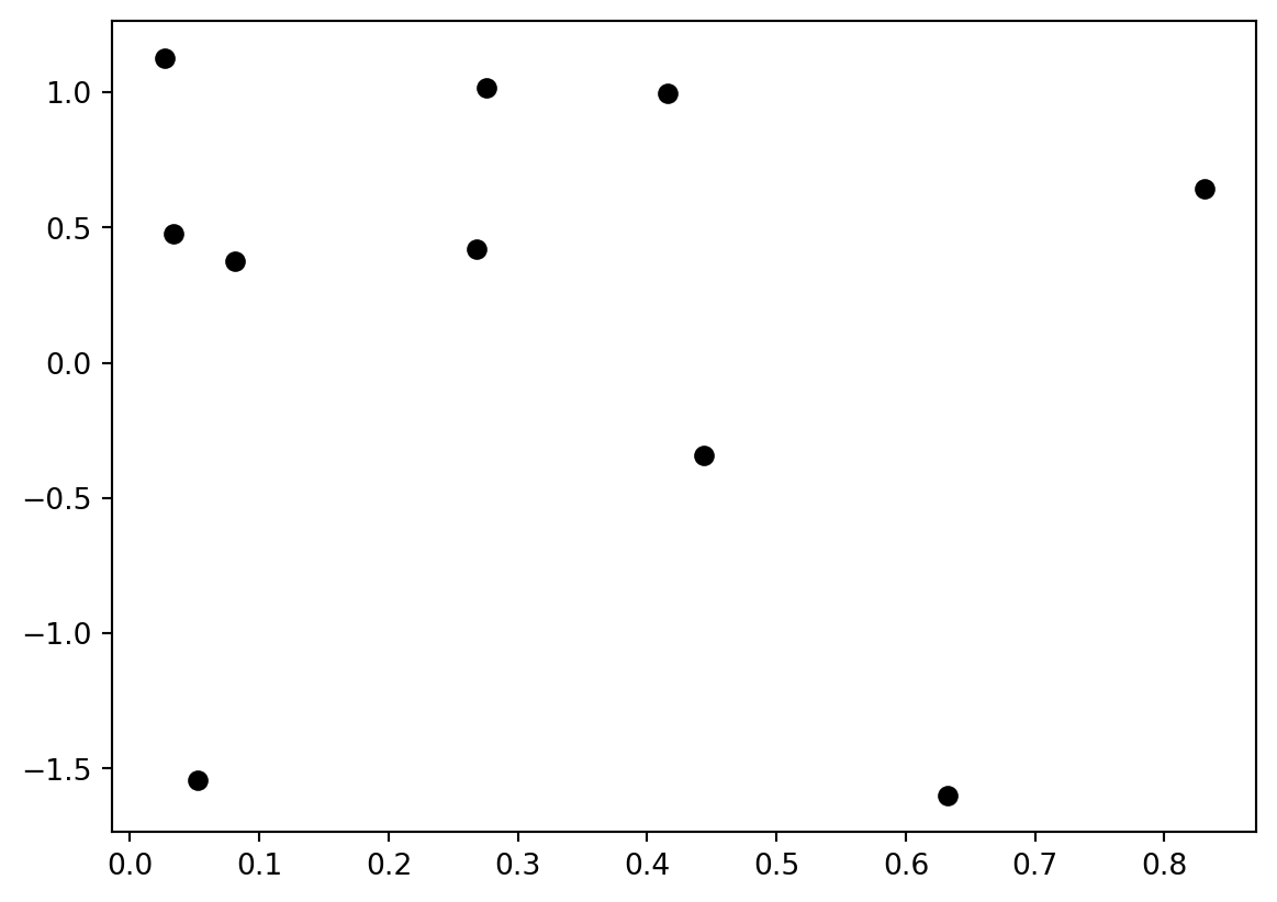

The string determines the plot appearance – in this case, black circles. You can use color strings (‘r’, ‘g’, ‘b’, ‘m’, ‘c’, ‘y’, …) or use the “Color” keyword to specify an RGB color. Marker appearance (‘o’,‘s’,‘v’,‘.’, …) controls how the points look.

If we connect those points using a line appearance specification (‘-’,‘–’,‘:’,…), it will not look very good, because the points are not ordered in any meaningful way. Let’s try a line plot using an ordered sequence of x values:

x_values = np.linspace(0,8,100)
y_values = np.sin(x_values)
plt.plot(x_values,y_values,'b');

This is actually a plot of a large number of points (100), with no marker shape and connected by a solid line.

For plotting multiple point sets or curves, you can pass more vectors into the plot function, or call the function multiple times:

x_values = np.linspace(0,8,100)
y1 = np.sin(x_values)         # sinusoidal function
y2 = (x_values - 3)**2 / 12   # a simple quadratic curve
y3 = 0.5*x_values - 1.0       # a simple linear function

plt.plot(x_values, y1, 'b-', x_values, y2, 'g--');  # plot two curves
plt.plot(x_values, y3, 'r:'); # add a curve to the plot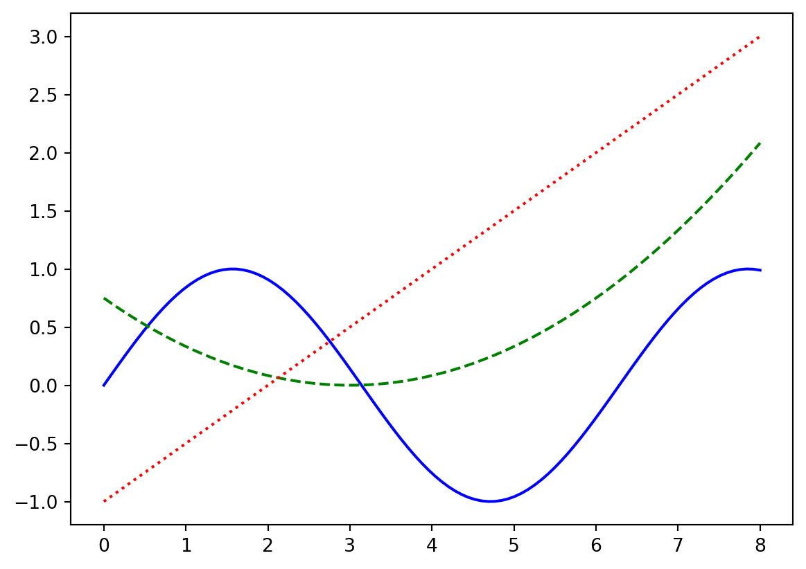

You may want to explicitly set the plot ranges – perhaps the most common pattern is to plot something, get the plot’s ranges, and then restore them later after plotting another function:

x_values = np.linspace(0,8,100)
y1 = np.sin(x_values)         # sinusoidal function
y3 = 0.5*x_values - 1.0       # a simple linear function

plt.plot(x_values, y1, 'b-') 
ax = plt.axis()               # get the x and y axis ranges
print(ax)
# now plot something else (which will change the axis ranges):
plt.plot(x_values, y3, 'r:'); # add the linear curve
plt.axis(ax);                 # restore the original plot's axis ranges

(np.float64(-0.4), np.float64(8.4), np.float64(-1.099652011574681), np.float64(1.0998559934443881))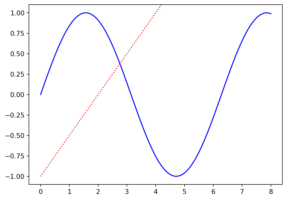

Legends

When plotting multiple point sets or curves we’ll likely want to be able to distinguish what each plot represents. We can do this by specifying a label for each plot, then adding a legend that tells us what each represents.

x_values = np.linspace(0,8,100)
y1 = np.sin(x_values)         # sinusoidal function
y2 = (x_values - 3)**2 / 12   # a simple quadratic curve
y3 = 0.5*x_values - 1.0       # a simple linear function

plt.plot(x_values, y1, 'b-', label='sin(x)');  # plot two curves
plt.plot(x_values, y2, 'g--', label='$(x-3)^2 / 12$')
plt.plot(x_values, y3, 'r:', label='$.5x-1$'); # add a curve to the plot
plt.legend();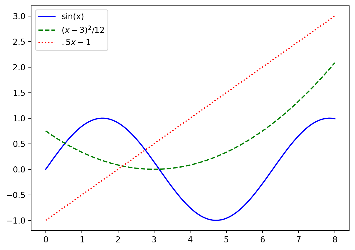

Here surrounding text in a label with $ $ allows us to write mathamatical equations as in LaTex!

Titles and labels

Typically we would like those viewing our plot to understand what the axes mean! We can label the x and y axes using plt.xlabel() and plt.ylabel() respectively. We can also set a title for our plot using plt.title()

x_values = np.linspace(0,8,100)
y = np.sin(x_values)          # sinusoidal function

plt.plot(x_values, y, 'b-');  # plot two curves
plt.xlabel('x')               # set the label for the x-axis
plt.ylabel('$sin(x)$')        # set the label for the y-axis
plt.title('x vs. $sin(x)$');  # set the title for the plot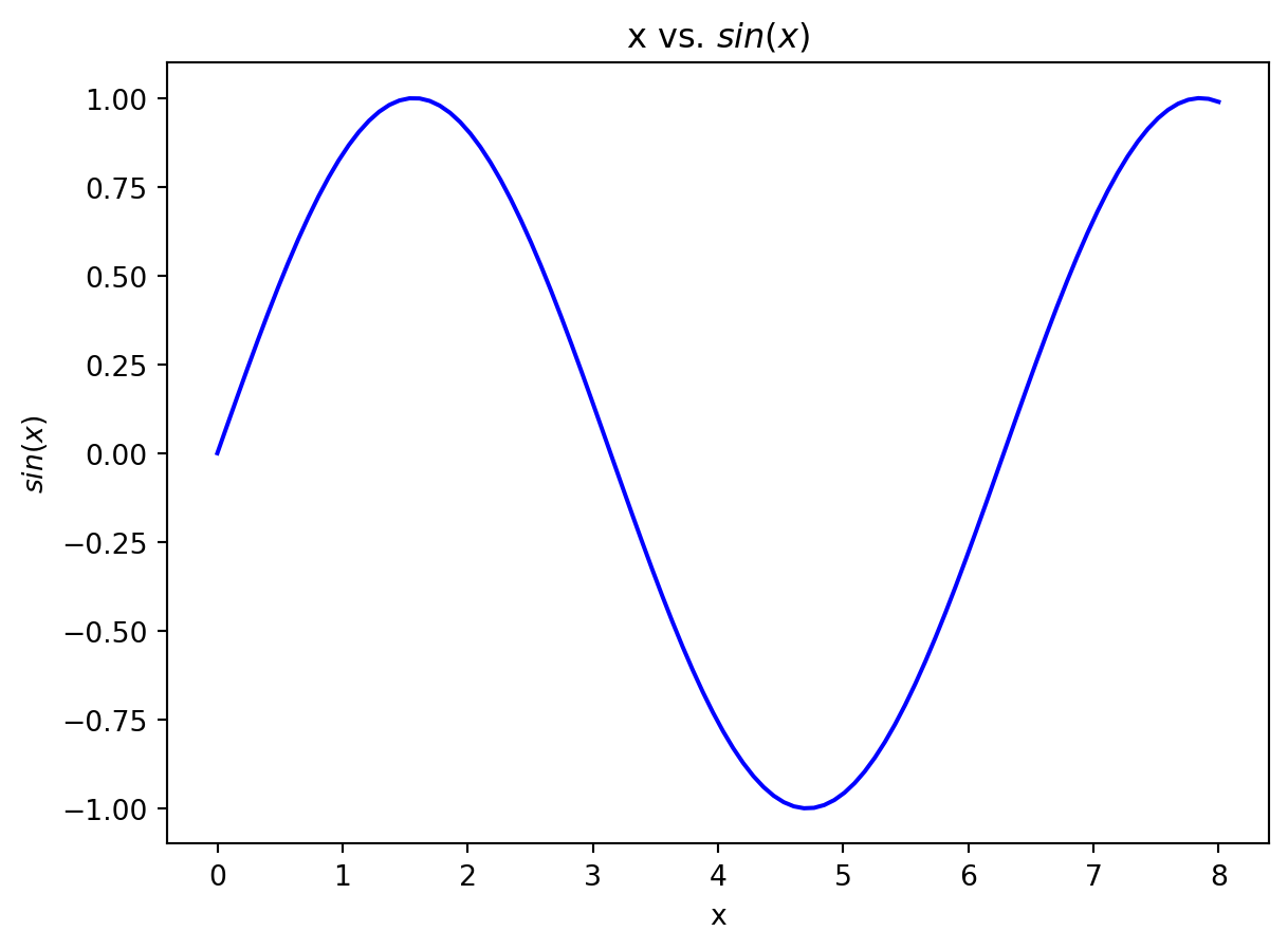

Histograms

Histograms are also useful visualizations:

plt.hist(y2, bins=20);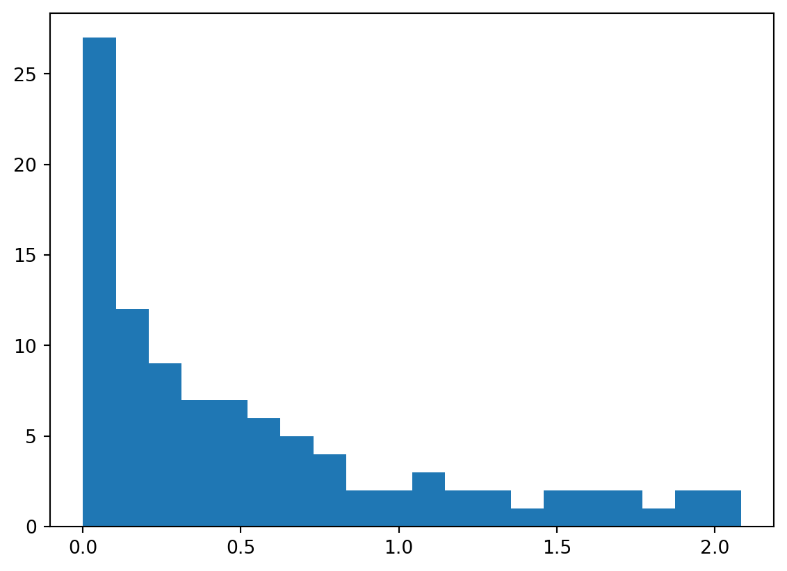

The outputs of hist include the bin locations, the number of data in each bin, and the “handles” to the plot elements to manipulate their appearance, if desired.

Subplots and plot sizes

It is often useful to put more than one plot together in a group; you can do this using the subplot function. There are various options; for example, “sharex” and “sharey” allow multiple plots to share a single axis range (or, you can set it manually, of course).

I often find it necessary to also change the geometry of the figure for multiple subplots – although this is more generally useful as well, if you have a plot that looks better wider and shorter, for example.

fig,ax = plt.subplots(1,3, figsize=(8.0, 2.0))      # make a 1 x 3 grid of plots:
ax[0].plot(x_values, y1, 'b-');   # plot y1 in the first subplot
ax[1].plot(x_values, y2, 'g--');  #   y2 in the 2nd
ax[2].plot(x_values, y3, 'r:');   #   and y3 in the last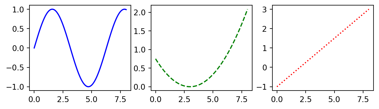

Subplot options

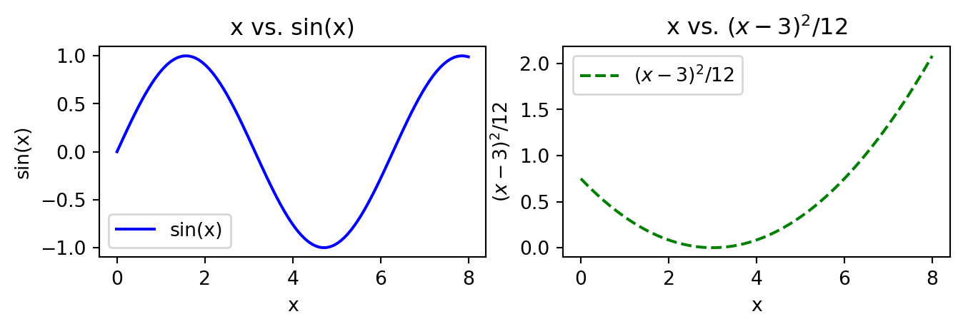
If we want to add legends or labeling to individual subplots we need to call methods of the individual subplot objects. In this case, the methods we need change a bit! Rather than using plt.title(), plt.xlabel() and plt.ylabel(), we need to use the methods ax.set_title(), ax.set_xlabel() and ax.set_ylabel()

fig,ax = plt.subplots(1,2, figsize=(8.0, 2.0))      # make a 1 x 3 grid of plots:
ax[0].plot(x_values, y1, 'b-', label='sin(x)');   # plot y1 in the first subplot
ax[1].plot(x_values, y2, 'g--', label='$(x-3)^2 / 12$');  #   y2 in the 2nd

# Add titles to both subplots
ax[0].set_title('x vs. sin(x)')
ax[1].set_title('x vs. $(x-3)^2 / 12$')

# Add axis labels
ax[0].set_xlabel('x')
ax[0].set_ylabel('sin(x)')

ax[1].set_xlabel('x')
ax[1].set_ylabel('$(x-3)^2 / 12$')

# Create legends for both subplots
ax[0].legend()
ax[1].legend();