Plot = import("https://esm.sh/@observablehq/plot")
d3 = require("d3@7")
topojson = require("topojson")
MathJax = require("https://cdnjs.cloudflare.com/ajax/libs/mathjax/3.2.2/es5/tex-svg.min.js").catch(() => window.MathJax)
tf = require("https://cdn.jsdelivr.net/npm/@tensorflow/tfjs@latest/dist/tf.min.js").catch(() => window.tf)

THREE = {
  const THREE = window.THREE = await require("three@0.130.0/build/three.min.js");
  await require("three@0.130.0/examples/js/controls/OrbitControls.js").catch(() => {});
  await require("three@0.130.0/examples/js/loaders/SVGLoader.js").catch(() => {});
  return THREE;
}

function sample(f, start, end, nsamples=100) {
  let arr = [...Array(nsamples).keys()]
  let dist = end - start
  function arrmap(ind) {
    const x = (ind * dist) / nsamples + start;
    return [x, f(x)];
  }
  return arr.map(arrmap)
}

function sigmoid(x){
  return 1 / (1 + Math.exp(-x));
}

function sum(x) {
  let s = 0;
  for (let i = 0; i < x.length; i++ ) {
    s += x[i];
  }
  return s;
}

function mean(x) {
  let s = 0;
  for (let i = 0; i < x.length; i++ ) {
    s += x[i];
  }
  return s / x.length;
}

function cross_ent(x, y) {
  return y ? -Math.log(sigmoid(x)) : -Math.log(sigmoid(-x));
}

function se(x, y) {
  return (x - y) * (x - y);
}

function shuffle(array) {
  let currentIndex = array.length,  randomIndex;

  // While there remain elements to shuffle.
  while (currentIndex > 0) {

    // Pick a remaining element.
    randomIndex = Math.floor(Math.random() * currentIndex);
    currentIndex--;

    // And swap it with the current element.
    [array[currentIndex], array[randomIndex]] = [
      array[randomIndex], array[currentIndex]];
  }

  return array;
}

function acc(x, y) {
  return Number(y == (x  > 0));
}

function grid_func(f, width, height, x1, y1, x2, y2) {
  let values = new Array(width * height);
  const xstride = (x2 - x1) / width;
  const ystride = (y2 - y1) / height;


  let y = 0;
  let x = 0;
  let ind = 0;
  for (let i = 0; i < height; i++ ) {
    for (let j = 0; j < width; j++, ind++) {
      x = x1 + j * xstride;
      y = y1 + i * ystride;
      values[ind] = f(x, y);
    }
  }
  return {width: width, height: height, x1: x1, y1: y1, x2: x2, y2: y2, values: values};
}

function get_accessors(keys, byindex=false) {
  let isString = value => typeof value === 'string';

  let index = 0;
  let indexmap = {};
  let accessors = [];
  for (let i = 0; i < keys.length; i++){
    let k = keys[i];
    if (Array.isArray(k)) {
      let access = isString(k[0]) ? (x => x[k[0]]) : k[0];

      if (byindex) {
        if (isString(k[0]) && !(k[0] in indexmap)) {
          indexmap[k[0]] = index;
          index++;
        }
        let accessindex = indexmap[k[0]];
        access = x => x[accessindex];
        let process = k[1];
        let final_access = x => process(access(x));
        accessors.push(final_access);
      }
      else {
        let process = k[1];
        let final_access = x => process(access(x));
        accessors.push(final_access);
      }

    }
    else {
      let access = isString(k) ? (x => x[k]) : k;
      if (byindex) {
        if (isString(k) && !(k in indexmap)) {
          indexmap[k] = index;
          index++;
        }
        let accessindex = indexmap[k];
        access = x => x[accessindex];
      }
      accessors.push(access);
    }
  }
  return accessors;
}

function predict(obs, weights, keys=["0", "1", "2", "3"], byindex=false) {
  let isString = value => typeof value === 'string';
  let accessors = get_accessors(keys, byindex);

  let output = weights[0];
  let wi = 1;
  for (let i = 0; (i < keys.length) && (wi < weights.length); i++, wi++){
    output += weights[wi] * accessors[i](obs);
  }
  return output;
}

function mean_loss(f, data, weights, keys, label, l2=0) {
  let reg = 0;
  if (l2 > 0){
    for (let i = 1; i < weights.length; i++) {
      reg += weights[i] * weights[i];
    }
  }

  const isString = value => typeof value === 'string';
  const get_label = isString(label) ? (x => x[label]) : label;
  return mean(data.map(x => f(predict(x, weights, keys), get_label(x)))) + l2 * reg;
}

function get_domains(data, accessors, margin=0.1) {
  let domains = [];
  for (let i = 0; i < accessors.length; i++){
    let xdomain = d3.extent(data, accessors[i]);
    let xdsize = (xdomain[1] - xdomain[0]);
    let xmin = xdomain[0] - xdsize * margin;
    let xmax = xdomain[1] + xdsize * margin;
    domains.push([xmin, xmax]);
  }
  return domains;
}

function logisticPlot2d(data, weights, keys, label, interval=0.05) {
  const accuracy = mean_loss(acc, data, weights, keys, label);

  let isString = value => typeof value === 'string';
  let accessors = get_accessors(keys);
  let index_accessors = get_accessors(keys, true);
  let domains = get_domains(data, accessors);
  const get_label = isString(label) ? (x => x[label]) : label;

  return Plot.plot({
    x: {tickSpacing: 80, label: "x"},
    y: {tickSpacing: 80, label: "y"},
    title: "Accuracy: " + accuracy.toFixed(3),
    color: {type: "linear", legend: true, scheme: "BuRd", domain: [-0.5, 1.5]},
    marks: [
      Plot.contour({
        fill: (x, y) => sigmoid(predict([x, y], weights, index_accessors)),
        x1: domains[0][0], y1: domains[1][0], x2: domains[0][1], y2: domains[1][1], interval: interval,
      }),
      Plot.dot(data, {x: accessors[0], y: accessors[1], stroke: x=> (get_label(x) ? 1.35 : -0.35)})
    ]
  });
}

function logisticLossPlot2d(data, weights, keys, label) {
  const loss = mean_loss(cross_ent, data, weights, keys, label);

  let isString = value => typeof value === 'string';
  let accessors = get_accessors(keys);
  let index_accessors = get_accessors(keys, true);
  let domains = get_domains(data, accessors);
  const get_label = isString(label) ? (x => x[label]) : label;

  return Plot.plot({
    x: {tickSpacing: 80, label: "x"},
    y: {tickSpacing: 80, label: "y"},
    title: "Loss: " + loss.toFixed(3),
    color: {type: "linear", legend: true, scheme: "BuRd", domain: [0, 5]},
    marks: [
      Plot.contour({
        value: (x, y) => predict([x, y], weights, index_accessors),
        fillOpacity: 0.2,
        stroke: "black", x1: domains[0][0], y1: domains[1][0], x2: domains[0][1], y2: domains[1][1],
        thresholds: [-1e6,  0, 0.00001]
      }),
      Plot.dot(data, {x: accessors[0], y: accessors[1], stroke: x=> cross_ent(predict(x, weights, keys), get_label(x)),
                      strokeOpacity: 0.5 })
    ]
  });
}

function lossPlot2d(f, data, keys, label, l2=0, res=100, x1=-40, y1=-0.015, x2=40,  y2=0.015, vmax=50, nlines=25, ctype="sqrt", scale=(x => x)) {
  let grid = 0;
  function lossFunc(w, b) {
    return scale(mean_loss(f, data, [w, b], keys, label, l2));
  }

  grid = grid_func(lossFunc,
                 res, res, x1, y1, x2, y2
                );

  function plot2d(weights) {
    let w = weights;
    if (!(Array.isArray(w[0]))){
      w = [w];
    }

    var arrows = w.slice(0, w.length - 1).map(function(e, i) {
      return e.concat(w[i+1]);
    });

    let interval= vmax / nlines;
    let thresholds = [];
    for (let i = 0; i < nlines; i++) {
      thresholds.push(i * interval);
    }
    let loss = mean_loss(f, data, w[w.length - 1], keys, label, l2)
    return Plot.plot({
      title: "Loss: " + loss.toFixed(3),
      color: {type: "linear", legend: true, label: "Loss", scheme: "BuRd", domain: [0, vmax], type: ctype},
      marks: [
        Plot.contour(grid.values, {width: grid.width, height: grid.height, x1: grid.x1, x2:grid.x2, y1: grid.y1, y2: grid.y2,
          stroke: Plot.identity, thresholds: thresholds}),
        Plot.dot(w),
        Plot.arrow(arrows, {x1: "0", y1: "1", x2: "2", y2: "3", stroke: "black"})
      ]
    })
  }
  return plot2d;
}


function regressionPlot(data, weights, keys, label, l2, f=se, stroke="") {
  let loss = mean_loss(f, data, weights, keys, label, l2);
  let isString = value => typeof value === 'string';

  let accessors = get_accessors(keys);
  let index_accessors = get_accessors(keys, true);
  let domains = get_domains(data, get_accessors([label].concat(keys)));
  const get_label = isString(label) ? (x => x[label]) : label;

  let stroke_shade = stroke;
  if (stroke == "") {
    stroke_shade = (x => f(predict(x, weights, keys), get_label(x)))
  }

  return Plot.plot({
    y: {domain: domains[0]},
    title: "Loss: " + loss.toFixed(3),
    color: {type: "linear", legend: true, label: "Loss", scheme: "BuRd", domain: [0, 100]},
    marks: [
      Plot.line(sample((x) => predict([x], weights, index_accessors), domains[1][0], domains[1][1]), {stroke: 'black'}),
      Plot.dot(data, {x: accessors[0], y: get_label, stroke: stroke_shade })
    ]
  })
}

function errorPlot(data, weights, keys, label, f, options={}) {
  const isString = value => typeof value === 'string';
  const get_label = isString(label) ? (x => x[label]) : label;
  let errors = data.map(x => [predict(x, weights, keys) - get_label(x), f(predict(x, weights, keys), get_label(x))]);


  let sigma = (options['sigma'] || 1);
  let plots = [];
  const xdomain = (options['xdomain'] || [-30, 30]);
  const ydomain = (options['ydomain'] || [0, 0.1]);


  if (options['plotnormal']){
    let pdf = x => Math.exp(-0.5 * x * x / sigma) * ydomain[1];
    let normal = Plot.line(sample(pdf, xdomain[0], xdomain[1]), {stroke: 'crimson'});
    plots.push(normal);
  }
  if (options['plotlaplace']){
    let pdf = x => Math.exp(-0.5 * Math.abs(x) / sigma) * ydomain[1];
    let normal = Plot.line(sample(pdf, xdomain[0], xdomain[1]), {stroke: 'green'});
    plots.push(normal);
  }

  return Plot.plot({
    y: {grid: true, domain: ydomain},
    x: {domain: xdomain},
    color: {type: "linear", legend: true, label: "Loss", scheme: "BuRd", domain: [0, 100]},
    marks: [
      //Plot.rectY(errors, Plot.binX({y: "count", fill: x => mean(x.map(v => v[1]))}, {x: "0"})),

      Plot.rectY(errors, Plot.binX({y: "proportion"}, {x: "0", fill: 'steelblue', interval: 1})),
      Plot.ruleY([0])
    ].concat(plots)
  })
}

function nnPlot(data, weights, keys, label, l2, f=se, stroke="", options=[]) {
  let loss = mean_loss(f, data, weights, keys, label, l2);
  let isString = value => typeof value === 'string';

  let accessors = get_accessors(keys);
  let index_accessors = get_accessors(keys, true);
  let domains = get_domains(data, get_accessors([label].concat(keys)));
  const get_label = isString(label) ? (x => x[label]) : label;

  let stroke_shade = stroke;
  if (stroke == "") {
    stroke_shade = (x => f(predict(x, weights, keys), get_label(x)))
  }

  let a = []
  if (options.indexOf("Show feature transforms") >= 0){
    a = [Plot.line(sample((x) =>  keys[1][1](x), domains[1][0], domains[1][1]), {stroke: 'red'}),
      Plot.line(sample((x) => keys[2][1](x), domains[1][0], domains[1][1]), {stroke: 'blue'})]
  }

  return Plot.plot({
    y: {domain: domains[0]},
    title: "Loss: " + loss.toFixed(3),
    color: {type: "linear", legend: true, label: "Loss", scheme: "BuRd", domain: [0, 100]},
    marks: [
      Plot.line(sample((x) => predict([x], weights, index_accessors), domains[1][0], domains[1][1]), {stroke: 'black'}),
      Plot.dot(data, {x: accessors[0], y: get_label, stroke: stroke_shade })
    ].concat(a)
  })
}Lecture 5: Neural networks
Neural networks
Background and a new visualization
So far in this class we have seen how to make predictions of some output \(y\) given an input \(\mathbf{x}\) using linear models. We saw that a reasonable model for continuous outputs \((y\in\mathbb{R})\) is linear regression.
\[ \textbf{Predict } y\in \textbf{ as } \begin{cases} y = \mathbf{x}^T\mathbf{w}\quad\quad\quad\quad\quad\quad\quad\quad\quad\quad\quad (\text{prediction function}) \\ \\ p(y\mid \mathbf{x}, \mathbf{w}, \sigma^2) = \mathcal{N}\big(y\mid \mathbf{x}^T\mathbf{w}, \sigma^2) \quad (\text{probabilistic view}) \end{cases} \]
A reasonable model for binary outputs \((y\in\{0,1\})\) is logistic regression:
\[ \textbf{Predict } y\in \textbf{ as } \begin{cases} y = \mathbb{I}(\mathbf{x}^T\mathbf{w} > 0)\ \quad\quad\quad\quad\quad (\text{prediction function}) \\ \\ p(y=1 \mid \mathbf{x}, \mathbf{w}) = \sigma(\mathbf{x}^T\mathbf{w}) \quad (\text{probabilistic view}) \end{cases} \]
A reasonable model for categorical outputs \((y\in\{0,1,…,C\})\) is multinomial logistic regression:
\[ \textbf{Predict } y\in \textbf{ as } \begin{cases} y = \underset{c}{\text{argmax}} \ \mathbf{x}^T\mathbf{w}_c \ \quad\quad\quad\quad\quad\quad\quad\ \ (\text{prediction function}) \\ \\ p(y=c \mid \mathbf{x}, \mathbf{w}) = \text{softmax}(\mathbf{x}^T\mathbf{W})_c \quad (\text{probabilistic view}) \end{cases} \]
In each of these cases, the core of our prediction is a linear function \((\mathbf{x}^T\mathbf{w})\) parameterized by a set of weights \(\mathbf{w}\), with possibly some nonlinear function (e.g. \(\sigma(\cdot)\)), applied to the result. This type of function is commonly depicted using a diagram like the one shown below.
Manim Community v0.18.1
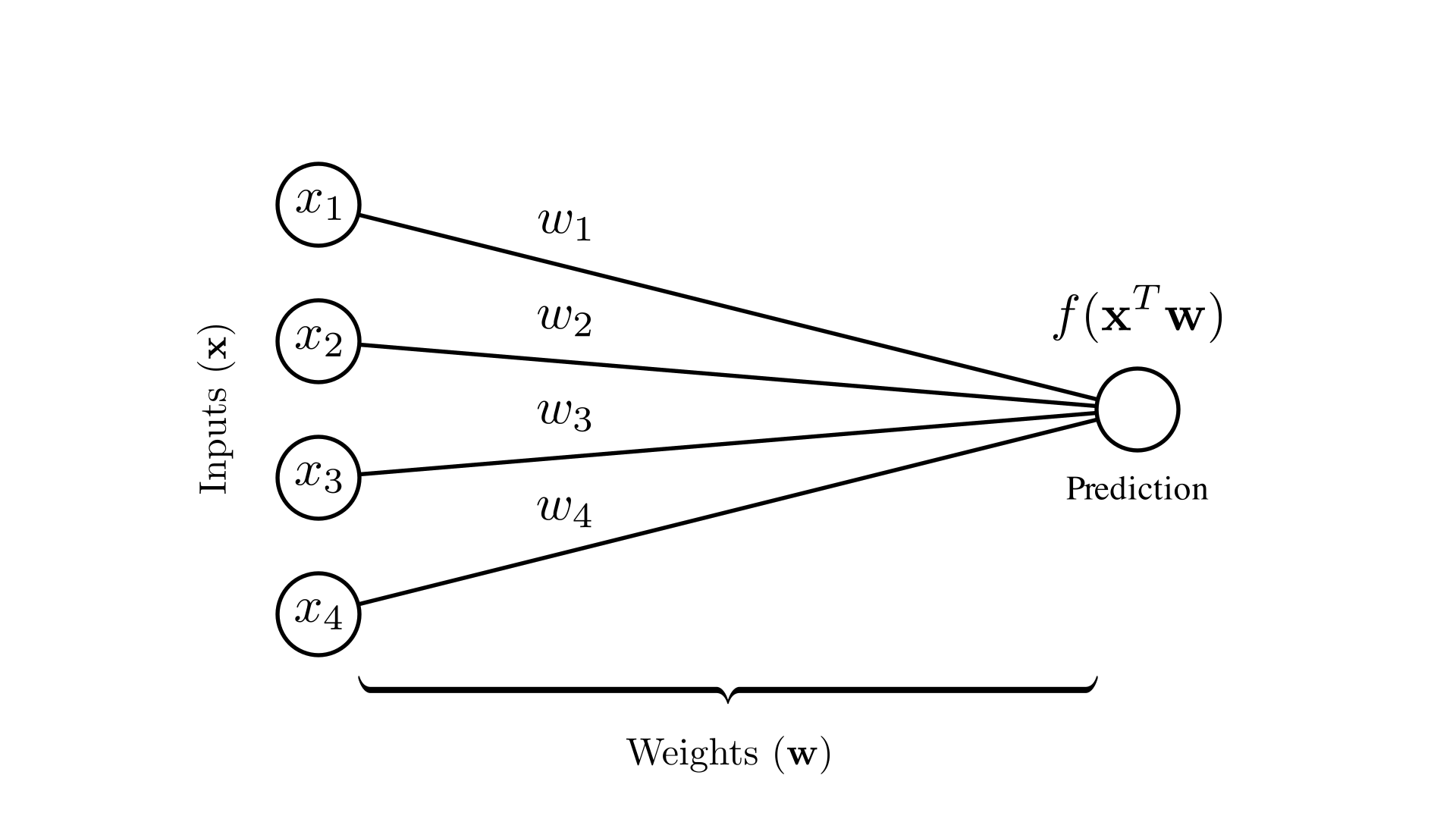
Each node corresponds to a scalar value: the nodes on the left correspond to each input dimension and the node on the right corresponds to the prediction. Each edge represents multiplying the value on the left with a corresponding weight.
Feature transforms revisited
In the last lecture we saw that we can define more complex and expressive functions by transforming the inputs in various ways. For example, we can define a function as:
\[ f(\mathbf{x})=\phi(\mathbf{x})^T \mathbf{w} ,\quad \phi(\mathbf{x}) = \begin{bmatrix} x_1 \\ x_2 \\ x_1^2 \\ x_2^2 \\ x_1x_2 \\ \sin(x_1) \\ \sin(x_2) \end{bmatrix} \]
Writing this out we get:
\[ f(\mathbf{x}) = w_1 x_1 + w_2 x_2 + w_3 x_1^2 + w_4 x_2^2 + w_5 x_1 x_2 + w_6 \sin(x_1) + w_7 \sin(x_2) \]
In code, we could consider transforming an entire dataset as follows:
squared_X = X ** 2              # x^2
cross_X = X[:, :1] * X[:, 1:2]  # x_1 * x_2
sin_X = np.sin(X)               # sin(x)

transformedX = np.concatenate([X, squared_X, cross_X, sin_X], axis=1)
Non-linear logistic regression
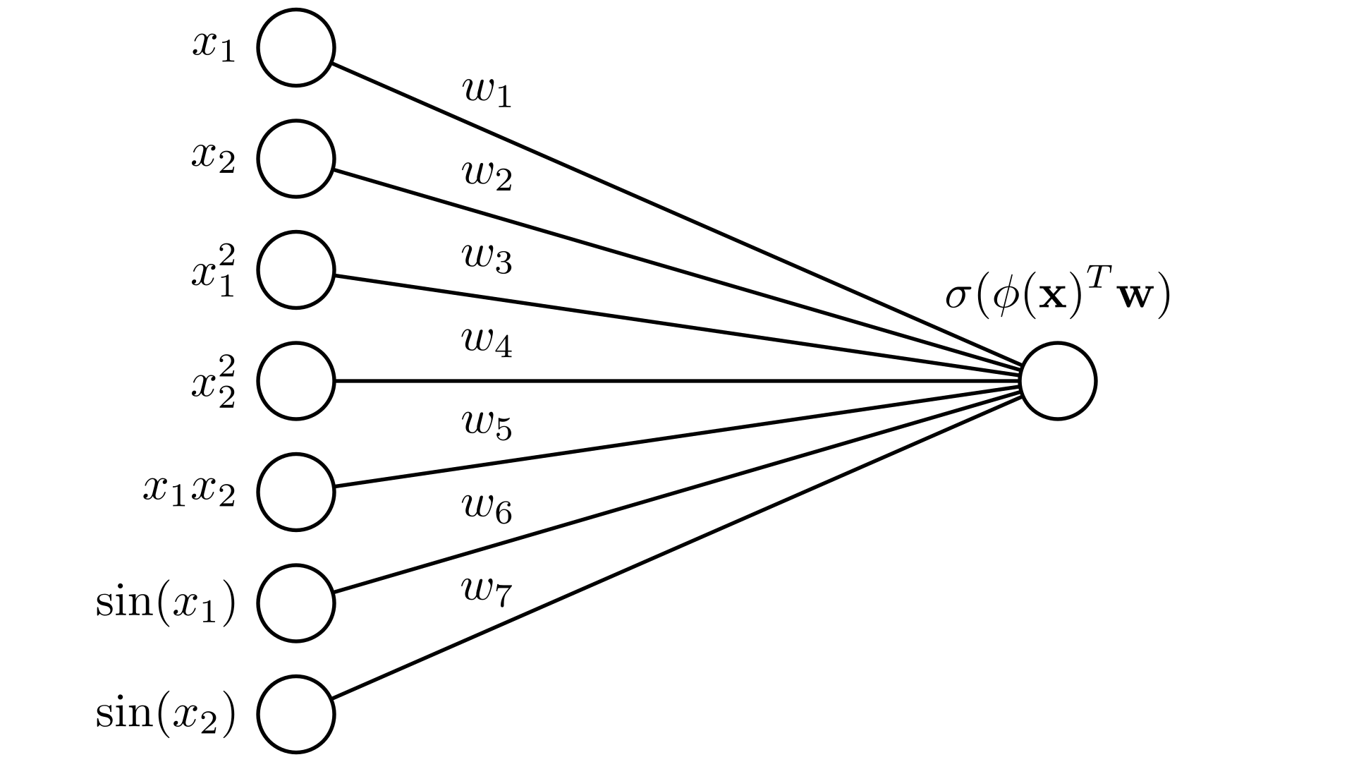
We can create a non-linear logistic regression model using the feature-transfor approach as:
\[ p(y=1\mid \mathbf{x}, \mathbf{w}) = \sigma\big( \phi(\mathbf{x})^T\mathbf{w} \big) \]
Pictorally, we can represent this using the diagram we just introduced as:
Manim Community v0.18.1
This demo application allows us to learn logistic regression models with different feature transforms. Hit the play button to start gradient descent!
This approach raises a big question though: how do we actually choose what transforms of our inputs to use?
Learned feature transforms
We’ve already seen that we can learn a function by defining our function in terms of a set of parameters \(\mathbf{w}\): \[f(\mathbf{x}) = \mathbf{x}^T\mathbf{w}\] and then minimizing a loss as a function of \(\mathbf{w}\) \[\mathbf{w}^* = \underset{\mathbf{w}}{\text{argmin}}\ \mathbf{Loss}(\mathbf{w})\] Which we can do with gradient descent: \[\mathbf{w}^{(k+1)} \longleftarrow \mathbf{w}^{(k)} - \alpha \nabla_{\mathbf{w}} \mathbf{Loss}(\mathbf{w})\]
So we didn’t choose \(\mathbf{w}\) explicitly, we let our algorithm find the optimal values. Ideally, we could do the same thing for our feature transforms: let our algorithm choose the optimal functions to use. This raises the question:
Can we learn the functions in our feature transform? The answer is yes! To see how, let’s start by writing out what this would look like. We’ll start with the feature transform framework we’ve already introduced, but now let’s replace the individual transforms with functions that we can learn.
\[ f(\mathbf{x})=\phi(\mathbf{x})^T \mathbf{w} ,\quad \phi(\mathbf{x}) = \begin{bmatrix} g_1(x_1) \\ g_2(x_1) \\ g_3(x_1) \\ g_4(x_1) \end{bmatrix} \]
The key insight we’ll use here is that we’ve already seen how to learn functions: this is exactly what our regression models are doing! So if we want to learn a feature transform, we can try using one of these functions that we know how to learn this case: logistic regression. \[g_i(\mathbf{x}) = \sigma(\mathbf{x}^T \mathbf{w}_i)\] With this form, we get a new feature transform: \[ f(\mathbf{x})=\phi(\mathbf{x})^T \mathbf{w}_0,\quad \phi(\mathbf{x}) = \begin{bmatrix} \sigma(\mathbf{x}^T \mathbf{w}_1) \\ \sigma(\mathbf{x}^T \mathbf{w}_2) \\ \sigma(\mathbf{x}^T \mathbf{w}_3) \\ \sigma(\mathbf{x}^T \mathbf{w}_4) \end{bmatrix} \]
Here we’ll call our original weight vector \(\mathbf{w}_0\) to distinguish it from the others. If we choose different weights for these different transform functions, we can have different feature transforms!
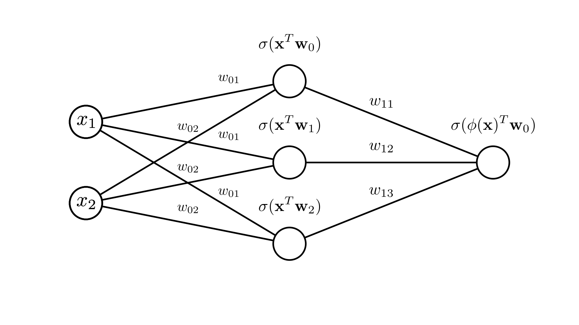
Let’s look at a very simple example: \[\mathbf{x} = \begin{bmatrix} x_1\\ x_2 \end{bmatrix}, \quad \mathbf{w}_0 = \begin{bmatrix} w_{01} \\ w_{02} \end{bmatrix}\] \[ f(\mathbf{x})=\phi(\mathbf{x})^T \mathbf{w}_0,\quad \phi(\mathbf{x}) = \begin{bmatrix} \sigma(\mathbf{x}^T \mathbf{w}_1) \\ \sigma(\mathbf{x}^T \mathbf{w}_2) \\ \sigma(\mathbf{x}^T \mathbf{w}_3) \end{bmatrix} = \begin{bmatrix} \sigma(x_1 w_{11} + x_2 w_{12}) \\ \sigma(x_1 w_{21} + x_2 w_{22}) \\ \sigma(x_1 w_{31} + x_2 w_{32}) \end{bmatrix} \]
In this case, we can write out our prediction function explicitly as: \[f(\mathbf{x}) = w_{01} \cdot\sigma(x_1 w_{11} + x_2 w_{12}) + w_{02} \cdot\sigma(x_1 w_{21} + x_2 w_{22})+ w_{03} \cdot\sigma(x_1 w_{31} + x_2 w_{32}) \]
We can represent this pictorially again as a node-link diagram:
Manim Community v0.18.1
We often omit the labels for compactness, which make it easy to draw larger models:
Neural networks
What we’ve just seen is a neural network!
Terminology-wise we call a single feature transform like \(\sigma(x_1 w_{11} + x_2 w_{12})\) a neuron.
We call the whole set of transformed features the hidden layer: \[\begin{bmatrix} \sigma(\mathbf{x}^T \mathbf{w}_1) \\ \sigma(\mathbf{x}^T \mathbf{w}_2) \\ \sigma(\mathbf{x}^T \mathbf{w}_3) \\ \sigma(\mathbf{x}^T \mathbf{w}_4) \end{bmatrix} \]
We call \(\mathbf{x}\) the input and \(f(\mathbf{x})\) the output.

Optimizing neural networks
We can still define a loss function for a neural network in the same way we did with our simpler linear models. The only difference is that now we have more parameters to choose:
\[ \mathbf{Loss}(\mathbf{w}_0,\mathbf{w}_1,\mathbf{w}_2,…) \]
Let’s look at the logistic regression negative log-likelihood loss for the simple neural network we saw above:
\[ p(y=1\mid \mathbf{x}, \mathbf{w}_0,\mathbf{w}_1,\mathbf{w}_2, \mathbf{w}_3)=\sigma(\phi(\mathbf{x})^T \mathbf{w}_0),\quad \phi(\mathbf{x}) = \begin{bmatrix} \sigma(\mathbf{x}^T \mathbf{w}_1) \\ \sigma(\mathbf{x}^T \mathbf{w}_2) \\ \sigma(\mathbf{x}^T \mathbf{w}_3) \end{bmatrix} \] \[ = \sigma\big(w_{01} \cdot\sigma(x_1 w_{11} + x_2 w_{12}) + w_{02} \cdot\sigma(x_1 w_{21} + x_2 w_{22})+ w_{03} \cdot\sigma(x_1 w_{31} + x_2 w_{32}) \big)\]
\[ \mathbf{NLL}(\mathbf{w}_0,..., \mathbf{X}, \mathbf{y}) = -\sum_{i=1}^N \bigg[ y_i\log p(y=1\mid \mathbf{x}, \mathbf{w}_0,...) + (1-y_i)\log p(y=0\mid \mathbf{x}, \mathbf{w}_0,...) \bigg] \]
We see that we can write out a full expression for this loss in term of all the inputs and weights. We can even define the gradient of this loss with respect to all the weights:
\[ \nabla_{\mathbf{w}_0...} = \begin{bmatrix} \frac{\partial \mathbf{NLL}}{\partial w_{01}} \\ \frac{\partial \mathbf{NLL}}{\partial w_{02}} \\ \frac{\partial \mathbf{NLL}}{\partial w_{03}} \\ \vdots\end{bmatrix} \]
While computing this gradient by hand would be tedious, this does mean we can update all of these weights as before using gradient descent! In future classes, we’ll look at how to automate the process of computing this gradient.
We can see this in action for this network here.
Neural networks with matrix notation
It is often more convenient to write all of the weights that are used to create our hidden layer as a single large matrix:
\[\mathbf{W}_1 = \begin{bmatrix} \mathbf{w}_1^T \\ \mathbf{w}_2^T \\ \mathbf{w}_3^T \\ \vdots \end{bmatrix}\] With this, we can write our general neural network more compactly as: \[f(\mathbf{x})= \sigma( \mathbf{W}_1 \mathbf{x})^T \mathbf{w_0} \] Or for a whole dataset: \[\mathbf{X} = \begin{bmatrix} \mathbf{x}_1^T \\ \mathbf{x}_2^T \\ \mathbf{x}_3^T \\ \vdots \end{bmatrix}\]
\[f(\mathbf{x})= \sigma( \mathbf{X}\mathbf{W}_1 )\mathbf{w_0}\]
Linear transforms
Thus far we’ve looked at a logistic regression feature transform as the basis of our neural network. Can we use linear regression as a feature transform?
Let’s see what happens in our simple example: \[\mathbf{x} = \begin{bmatrix} x_1\\ x_2 \end{bmatrix}, \quad \mathbf{w}_0 = \begin{bmatrix} w_{01} \\ w_{02} \end{bmatrix}\] \[ f(\mathbf{x})=\phi(\mathbf{x})^T \mathbf{w}_0,\quad \phi(\mathbf{x}) = \begin{bmatrix} \mathbf{x}^T \mathbf{w}_1 \\ \mathbf{x}^T \mathbf{w}_2 \\ \mathbf{x}^T \mathbf{w}_3 \\ \end{bmatrix} = \begin{bmatrix} x_1 w_{11} + x_2 w_{12} \\ x_1 w_{21} + x_2 w_{22} \\ x_1 w_{31} + x_2 w_{32} \\\end{bmatrix} \] In this case, we can write out our prediction function explicitly as: \[f(\mathbf{x}) = w_{01}\cdot (x_1 w_{11} + x_2 w_{12}) + w_{02} \cdot(x_1 w_{21} + x_2 w_{22})+ w_{03} \cdot(x_1 w_{31} + x_2 w_{32}) \] \[= (w_{11}w_{01}) x_1 +(w_{12}w_{01}) x_2 + (w_{21}w_{02}) x_1 +(w_{22}w_{02}) x_2 +(w_{31}w_{03}) x_1 +(w_{32}w_{03}) x_2 \]
\[ = (w_{11}w_{01} + w_{21}w_{02} + w_{31}w_{03}) x_1 + (w_{12}w_{01} + w_{22} w_{02} + w_{32} w_{03}) x_2 \]
We see that we ultimately just end up with another linear function of \(\mathbf{x}\) and we’re no better off than in our orginal case. We can see this in practice here.
In general: \[ f(\mathbf{x})=\phi(\mathbf{x})^T \mathbf{w}_0,\quad \phi(\mathbf{x}) = \begin{bmatrix} \mathbf{x}^T \mathbf{w}_1 \\ \mathbf{x}^T \mathbf{w}_2\\ \mathbf{x}^T \mathbf{w}_3 \\ \mathbf{x}^T \mathbf{w}_4\end{bmatrix} \]
\[ f(\mathbf{x})= w_{01} (\mathbf{x}^T \mathbf{w}_1) + w_{02} (\mathbf{x}^T \mathbf{w}_2) +... \] \[= \mathbf{x}^T ( w_{01}\mathbf{w}_1) + \mathbf{x}^T (w_{02} \mathbf{w}_2) +... \] Which is again just a linear function. The motivates the need for using a non-linear function like \(\sigma(\cdot)\) in our neurons.
Activation functions
While we need a non-linear function as part of our neural network feature transform, it does not need to be the sigmoid function. A few other common choices are:
\[ \textbf{Sigmoid:}\quad \sigma(x) = \frac{1}{1+e^{-x}} \]
\[ \textbf{Hyperbolic tangent:}\quad \tanh(x) = \frac{e^{2x}-1}{e^{2x}+1} \]
\[ \textbf{Rectifed linear:}\quad \text{ReLU}(x) = \max(x,\ 0) \]
Manim Community v0.18.1
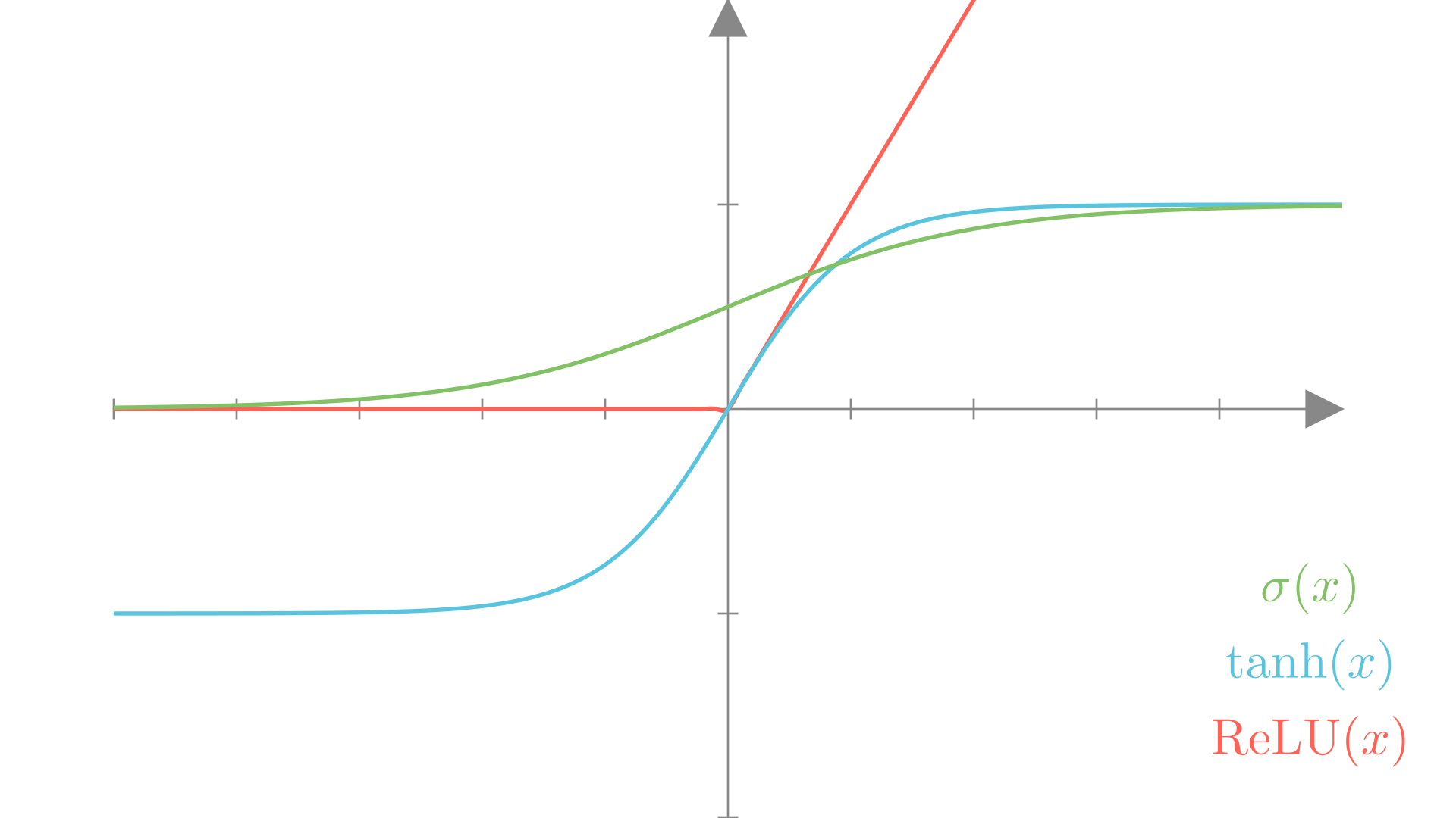
We call these non-linear functions activation functions when used in neural networks. We’ll see other examples over the course of this class
Try out different activation functions here.
Multi-layer neural networks
What we’ve seen so far is a single hidden-layer neural network. But there’s no reason we’re restricted to a single layer!