Plot = import("https://esm.sh/@observablehq/plot")
d3 = require("d3@7")
topojson = require("topojson")
MathJax = require("https://cdnjs.cloudflare.com/ajax/libs/mathjax/3.2.2/es5/tex-svg.min.js").catch(() => window.MathJax)
tf = require("https://cdn.jsdelivr.net/npm/@tensorflow/tfjs@latest/dist/tf.min.js").catch(() => window.tf)

THREE = {
  const THREE = window.THREE = await require("three@0.130.0/build/three.min.js");
  await require("three@0.130.0/examples/js/controls/OrbitControls.js").catch(() => {});
  await require("three@0.130.0/examples/js/loaders/SVGLoader.js").catch(() => {});
  return THREE;
}

function sample(f, start, end, nsamples=100) {
  let arr = [...Array(nsamples).keys()]
  let dist = end - start
  function arrmap(ind) {
    const x = (ind * dist) / nsamples + start;
    return [x, f(x)];
  }
  return arr.map(arrmap)
}

function sigmoid(x){
  return 1 / (1 + Math.exp(-x));
}

function sum(x) {
  let s = 0;
  for (let i = 0; i < x.length; i++ ) {
    s += x[i];
  }
  return s;
}

function mean(x) {
  let s = 0;
  for (let i = 0; i < x.length; i++ ) {
    s += x[i];
  }
  return s / x.length;
}

function cross_ent(x, y) {
  return y ? -Math.log(sigmoid(x)) : -Math.log(sigmoid(-x));
}

function se(x, y) {
  return (x - y) * (x - y);
}

function shuffle(array) {
  let currentIndex = array.length,  randomIndex;

  // While there remain elements to shuffle.
  while (currentIndex > 0) {

    // Pick a remaining element.
    randomIndex = Math.floor(Math.random() * currentIndex);
    currentIndex--;

    // And swap it with the current element.
    [array[currentIndex], array[randomIndex]] = [
      array[randomIndex], array[currentIndex]];
  }

  return array;
}

function acc(x, y) {
  return Number(y == (x  > 0));
}

function grid_func(f, width, height, x1, y1, x2, y2) {
  let values = new Array(width * height);
  const xstride = (x2 - x1) / width;
  const ystride = (y2 - y1) / height;


  let y = 0;
  let x = 0;
  let ind = 0;
  for (let i = 0; i < height; i++ ) {
    for (let j = 0; j < width; j++, ind++) {
      x = x1 + j * xstride;
      y = y1 + i * ystride;
      values[ind] = f(x, y);
    }
  }
  return {width: width, height: height, x1: x1, y1: y1, x2: x2, y2: y2, values: values};
}

function get_accessors(keys, byindex=false) {
  let isString = value => typeof value === 'string';

  let index = 0;
  let indexmap = {};
  let accessors = [];
  for (let i = 0; i < keys.length; i++){
    let k = keys[i];
    if (Array.isArray(k)) {
      let access = isString(k[0]) ? (x => x[k[0]]) : k[0];

      if (byindex) {
        if (isString(k[0]) && !(k[0] in indexmap)) {
          indexmap[k[0]] = index;
          index++;
        }
        let accessindex = indexmap[k[0]];
        access = x => x[accessindex];
        let process = k[1];
        let final_access = x => process(access(x));
        accessors.push(final_access);
      }
      else {
        let process = k[1];
        let final_access = x => process(access(x));
        accessors.push(final_access);
      }

    }
    else {
      let access = isString(k) ? (x => x[k]) : k;
      if (byindex) {
        if (isString(k) && !(k in indexmap)) {
          indexmap[k] = index;
          index++;
        }
        let accessindex = indexmap[k];
        access = x => x[accessindex];
      }
      accessors.push(access);
    }
  }
  return accessors;
}

function predict(obs, weights, keys=["0", "1", "2", "3"], byindex=false) {
  let isString = value => typeof value === 'string';
  let accessors = get_accessors(keys, byindex);

  let output = weights[0];
  let wi = 1;
  for (let i = 0; (i < keys.length) && (wi < weights.length); i++, wi++){
    output += weights[wi] * accessors[i](obs);
  }
  return output;
}

function mean_loss(f, data, weights, keys, label, l2=0) {
  let reg = 0;
  if (l2 > 0){
    for (let i = 1; i < weights.length; i++) {
      reg += weights[i] * weights[i];
    }
  }

  const isString = value => typeof value === 'string';
  const get_label = isString(label) ? (x => x[label]) : label;
  return mean(data.map(x => f(predict(x, weights, keys), get_label(x)))) + l2 * reg;
}

function get_domains(data, accessors, margin=0.1) {
  let domains = [];
  for (let i = 0; i < accessors.length; i++){
    let xdomain = d3.extent(data, accessors[i]);
    let xdsize = (xdomain[1] - xdomain[0]);
    let xmin = xdomain[0] - xdsize * margin;
    let xmax = xdomain[1] + xdsize * margin;
    domains.push([xmin, xmax]);
  }
  return domains;
}

function logisticPlot2d(data, weights, keys, label, interval=0.05) {
  const accuracy = mean_loss(acc, data, weights, keys, label);

  let isString = value => typeof value === 'string';
  let accessors = get_accessors(keys);
  let index_accessors = get_accessors(keys, true);
  let domains = get_domains(data, accessors);
  const get_label = isString(label) ? (x => x[label]) : label;

  return Plot.plot({
    x: {tickSpacing: 80, label: "x"},
    y: {tickSpacing: 80, label: "y"},
    title: "Accuracy: " + accuracy.toFixed(3),
    color: {type: "linear", legend: true, scheme: "BuRd", domain: [-0.5, 1.5]},
    marks: [
      Plot.contour({
        fill: (x, y) => sigmoid(predict([x, y], weights, index_accessors)),
        x1: domains[0][0], y1: domains[1][0], x2: domains[0][1], y2: domains[1][1], interval: interval,
      }),
      Plot.dot(data, {x: accessors[0], y: accessors[1], stroke: x=> (get_label(x) ? 1.35 : -0.35)})
    ]
  });
}

function logisticLossPlot2d(data, weights, keys, label) {
  const loss = mean_loss(cross_ent, data, weights, keys, label);

  let isString = value => typeof value === 'string';
  let accessors = get_accessors(keys);
  let index_accessors = get_accessors(keys, true);
  let domains = get_domains(data, accessors);
  const get_label = isString(label) ? (x => x[label]) : label;

  return Plot.plot({
    x: {tickSpacing: 80, label: "x"},
    y: {tickSpacing: 80, label: "y"},
    title: "Loss: " + loss.toFixed(3),
    color: {type: "linear", legend: true, scheme: "BuRd", domain: [0, 5]},
    marks: [
      Plot.contour({
        value: (x, y) => predict([x, y], weights, index_accessors),
        fillOpacity: 0.2,
        stroke: "black", x1: domains[0][0], y1: domains[1][0], x2: domains[0][1], y2: domains[1][1],
        thresholds: [-1e6,  0, 0.00001]
      }),
      Plot.dot(data, {x: accessors[0], y: accessors[1], stroke: x=> cross_ent(predict(x, weights, keys), get_label(x)),
                      strokeOpacity: 0.5 })
    ]
  });
}

function lossPlot2d(f, data, keys, label, l2=0, res=100, x1=-40, y1=-0.015, x2=40,  y2=0.015, vmax=50, nlines=25, ctype="sqrt", scale=(x => x)) {
  let grid = 0;
  function lossFunc(w, b) {
    return scale(mean_loss(f, data, [w, b], keys, label, l2));
  }

  grid = grid_func(lossFunc,
                 res, res, x1, y1, x2, y2
                );

  function plot2d(weights) {
    let w = weights;
    if (!(Array.isArray(w[0]))){
      w = [w];
    }

    var arrows = w.slice(0, w.length - 1).map(function(e, i) {
      return e.concat(w[i+1]);
    });

    let interval= vmax / nlines;
    let thresholds = [];
    for (let i = 0; i < nlines; i++) {
      thresholds.push(i * interval);
    }
    let loss = mean_loss(f, data, w[w.length - 1], keys, label, l2)
    return Plot.plot({
      title: "Loss: " + loss.toFixed(3),
      color: {type: "linear", legend: true, label: "Loss", scheme: "BuRd", domain: [0, vmax], type: ctype},
      marks: [
        Plot.contour(grid.values, {width: grid.width, height: grid.height, x1: grid.x1, x2:grid.x2, y1: grid.y1, y2: grid.y2,
          stroke: Plot.identity, thresholds: thresholds}),
        Plot.dot(w),
        Plot.arrow(arrows, {x1: "0", y1: "1", x2: "2", y2: "3", stroke: "black"})
      ]
    })
  }
  return plot2d;
}


function regressionPlot(data, weights, keys, label, l2, f=se, stroke="") {
  let loss = mean_loss(f, data, weights, keys, label, l2);
  let isString = value => typeof value === 'string';

  let accessors = get_accessors(keys);
  let index_accessors = get_accessors(keys, true);
  let domains = get_domains(data, get_accessors([label].concat(keys)));
  const get_label = isString(label) ? (x => x[label]) : label;

  let stroke_shade = stroke;
  if (stroke == "") {
    stroke_shade = (x => f(predict(x, weights, keys), get_label(x)))
  }

  return Plot.plot({
    y: {domain: domains[0]},
    title: "Loss: " + loss.toFixed(3),
    color: {type: "linear", legend: true, label: "Loss", scheme: "BuRd", domain: [0, 100]},
    marks: [
      Plot.line(sample((x) => predict([x], weights, index_accessors), domains[1][0], domains[1][1]), {stroke: 'black'}),
      Plot.dot(data, {x: accessors[0], y: get_label, stroke: stroke_shade })
    ]
  })
}

function errorPlot(data, weights, keys, label, f, options={}) {
  const isString = value => typeof value === 'string';
  const get_label = isString(label) ? (x => x[label]) : label;
  let errors = data.map(x => [predict(x, weights, keys) - get_label(x), f(predict(x, weights, keys), get_label(x))]);


  let sigma = (options['sigma'] || 1);
  let plots = [];
  const xdomain = (options['xdomain'] || [-30, 30]);
  const ydomain = (options['ydomain'] || [0, 0.1]);


  if (options['plotnormal']){
    let pdf = x => Math.exp(-0.5 * x * x / sigma) * ydomain[1];
    let normal = Plot.line(sample(pdf, xdomain[0], xdomain[1]), {stroke: 'crimson'});
    plots.push(normal);
  }
  if (options['plotlaplace']){
    let pdf = x => Math.exp(-0.5 * Math.abs(x) / sigma) * ydomain[1];
    let normal = Plot.line(sample(pdf, xdomain[0], xdomain[1]), {stroke: 'green'});
    plots.push(normal);
  }

  return Plot.plot({
    y: {grid: true, domain: ydomain},
    x: {domain: xdomain},
    color: {type: "linear", legend: true, label: "Loss", scheme: "BuRd", domain: [0, 100]},
    marks: [
      //Plot.rectY(errors, Plot.binX({y: "count", fill: x => mean(x.map(v => v[1]))}, {x: "0"})),

      Plot.rectY(errors, Plot.binX({y: "proportion"}, {x: "0", fill: 'steelblue', interval: 1})),
      Plot.ruleY([0])
    ].concat(plots)
  })
}

function nnPlot(data, weights, keys, label, l2, f=se, stroke="", options=[]) {
  let loss = mean_loss(f, data, weights, keys, label, l2);
  let isString = value => typeof value === 'string';

  let accessors = get_accessors(keys);
  let index_accessors = get_accessors(keys, true);
  let domains = get_domains(data, get_accessors([label].concat(keys)));
  const get_label = isString(label) ? (x => x[label]) : label;

  let stroke_shade = stroke;
  if (stroke == "") {
    stroke_shade = (x => f(predict(x, weights, keys), get_label(x)))
  }

  let a = []
  if (options.indexOf("Show feature transforms") >= 0){
    a = [Plot.line(sample((x) =>  keys[1][1](x), domains[1][0], domains[1][1]), {stroke: 'red'}),
      Plot.line(sample((x) => keys[2][1](x), domains[1][0], domains[1][1]), {stroke: 'blue'})]
  }

  return Plot.plot({
    y: {domain: domains[0]},
    title: "Loss: " + loss.toFixed(3),
    color: {type: "linear", legend: true, label: "Loss", scheme: "BuRd", domain: [0, 100]},
    marks: [
      Plot.line(sample((x) => predict([x], weights, index_accessors), domains[1][0], domains[1][1]), {stroke: 'black'}),
      Plot.dot(data, {x: accessors[0], y: get_label, stroke: stroke_shade })
    ].concat(a)
  })
}Lecture 6: Deep neural networks and backpropagation
Neural networks
Neural networks with matrices
Let’s return to our simple neural network example, where we have 2 inputs and 3 neurons (transforms): \[\mathbf{x} = \begin{bmatrix} x_1\\ x_2 \end{bmatrix}, \quad \mathbf{w}_0 = \begin{bmatrix} w_{01} \\ w_{02} \end{bmatrix}\] \[ f(\mathbf{x})=\phi(\mathbf{x})^T \mathbf{w}_0,\quad \phi(\mathbf{x}) = \begin{bmatrix} \sigma(\mathbf{x}^T \mathbf{w}_1) \\ \sigma(\mathbf{x}^T \mathbf{w}_2) \\ \sigma(\mathbf{x}^T \mathbf{w}_3) \end{bmatrix} = \begin{bmatrix} \sigma(x_1 w_{11} + x_2 w_{12}) \\ \sigma(x_1 w_{21} + x_2 w_{22}) \\ \sigma(x_1 w_{31} + x_2 w_{32}) \end{bmatrix} \]
Again, we can represent this pictorially again as a node-link diagram:
Manim Community v0.18.1

Let’s look at a more compact way to write this, using a weight matrix for the neural network layer. Let’s look at the transform before we apply the sigmoid function:
\[ \begin{bmatrix} \mathbf{x}^T \mathbf{w}_1 \\ \mathbf{x}^T \mathbf{w}_2 \\ \mathbf{x}^T \mathbf{w}_3 \end{bmatrix} = \begin{bmatrix} x_1 w_{11} + x_2 w_{12} \\ x_1 w_{21} + x_2 w_{22} \\ x_1 w_{31} + x_2 w_{32} \end{bmatrix} = \begin{bmatrix} w_{11} & w_{12} \\w_{21} & w_{22} \\ w_{31} & w_{32} \end{bmatrix} \begin{bmatrix} x_1 \\ x_2 \end{bmatrix} \]
If we define a matrix \(\mathbf{W}\) for all of the weights as:
\[ \mathbf{W} = \begin{bmatrix} w_{11} & w_{12} \\w_{21} & w_{22} \\ w_{31} & w_{32} \end{bmatrix} \]
we get:
\[
\begin{bmatrix} \mathbf{x}^T \mathbf{w}_1 \\ \mathbf{x}^T \mathbf{w}_2 \\ \mathbf{x}^T \mathbf{w}_3 \end{bmatrix} = \mathbf{W}\mathbf{x} = (\mathbf{x}^T\mathbf{W}^T)^T
\]
If we let \(h\) be the number of neuron (or hidden layer units) then this is a \(h \times d\) matrix. Therefore, we can write our transform as:
\[ \phi(\mathbf{x}) = \sigma(\mathbf{x}^T\mathbf{W}^T)^T, \quad f(\mathbf{x}) = \sigma(\mathbf{x}^T\mathbf{W}^T) \mathbf{w}_0 \]
Recall that if we have multiple observations, as in a dataset, we define them together as an \(N \times d\) matrix \(\mathbf{X}\) such that each row is an observation:
\[ \mathbf{X} = \begin{bmatrix} \mathbf{x}_1^T \\ \mathbf{x}_2^T \\ \mathbf{x}_3^T \\ \vdots \end{bmatrix} \]
Therefore, we can transform all of these observations at once by multiplying this matrix by \(\mathbf{W}^T\).
\[ \phi(\mathbf{X}) = \sigma(\mathbf{X}\mathbf{W}^T)^T = \begin{bmatrix} \sigma(\mathbf{x}_1^T\mathbf{w}_1) & \sigma(\mathbf{x}_1^T\mathbf{w}_2) & \dots & \sigma(\mathbf{x}_1^T\mathbf{w}_h \\ \sigma(\mathbf{x}_2^T\mathbf{w}_1) & \sigma(\mathbf{x}_2^T\mathbf{w}_2) & \dots & \sigma(\mathbf{x}_2^T\mathbf{w}_h) \\ \vdots & \vdots & \ddots & \vdots \\ \sigma(\mathbf{x}_N^T\mathbf{w}_1) & \sigma(\mathbf{x}_N^T\mathbf{w}_2) & \dots & \sigma(\mathbf{x}_N^T\mathbf{w}_h) \end{bmatrix} \]
We see that this is an \(N \times h\) matrix where each row is a transformed observation! We can then write our full prediction function as
\[ \quad f(\mathbf{x}) = \sigma(\mathbf{X}\mathbf{W}^T) \mathbf{w}_0 \]
To summarize:
\(\mathbf{X}: \quad N \times d\) matrix of observations
\(\mathbf{W}: \quad h \times d\) matrix of network weights
\(\mathbf{w}_0: \quad h\ (\times 1)\) vector of linear regression weights
If we check that our dimensions work for matrix multiplication we see that we get the \(N\times 1\) vector of predictions we are looking for!
\[ (N \times d) (h \times d)^T (h \times 1) \rightarrow (N \times d) (d \times h) (h \times 1) \rightarrow (N \times h) (h \times 1) \]
\[ \longrightarrow (N \times1) \]
Benefits of neural networks
We’ve seen that the neural network transform is still fairly restrictive, with a limited number of neurons we can’t fit any arbitrary function. In fact, if we choose our feature transforms wisely we can do better than than a neural network.
For example, consider the simple 3-neuron network above. We can see that if we try to fit a circular dataset with it, it performs worse than an explicit transform with \(x_1^2\) and \(x_2^2\).
Circle dataset with \(x_1^2\) and \(x_2^2\):
Similarly, for a cross dataset, we can do better with the feature transform that includes \(x_1x_2\) as a feature:
However, if we choose the wrong feature transform for a given dataset, we do far worse.
Circle dataset with \(x_1 x_2\)
Cross dataset with \(x_1^2\) and \(x_2^2\)
We see that the real power of the neural network here is the ability to adapt the transform to the given dataset, without needing to carefully choose the correct transform!
Deep Neural Networks
What we’ve seen so far is a neural network with a single hidden layer, meaning that we create a feature transform for our data and then simply use that to make our prediction. We see that each individual feature transform is a bit limited, being just a logistic regression function.
\[\phi(\mathbf{x})_i = \sigma(\mathbf{x}^T \mathbf{w}_i)\]
No matter what we set \(\mathbf{w}_i\) this transform would not be able to replicate a transform like \(\phi(\mathbf{x})_i = x_i^2\). However, we’ve already seen a way to make logistic regression more expressive: neural networks!
The idea behind a deep or multi-layer neural network is that we can apply this idea of neural network feature transforms recursively:
\[\phi(\mathbf{x})_i = \sigma(\sigma(\mathbf{x}^T\mathbf{W}^T) \mathbf{w}_i)\]
Here we’ve transformed our input before computing our feature transform. In terms of a dataset we can write the full prediction function for this 2-layer network as:
\[ f(\mathbf{X}) = \sigma(\sigma(\mathbf{X}\mathbf{W}_1^T)\mathbf{W}_2^T)\mathbf{w}_0 \]
We’ve now defined a set of weight parameters for each of our 2 hidden layers \(\mathbf{W}_1\) and \(\mathbf{W}_2\). It’s a little easier to see what’s happening here if we look a our diagram for this case:
Manim Community v0.18.1
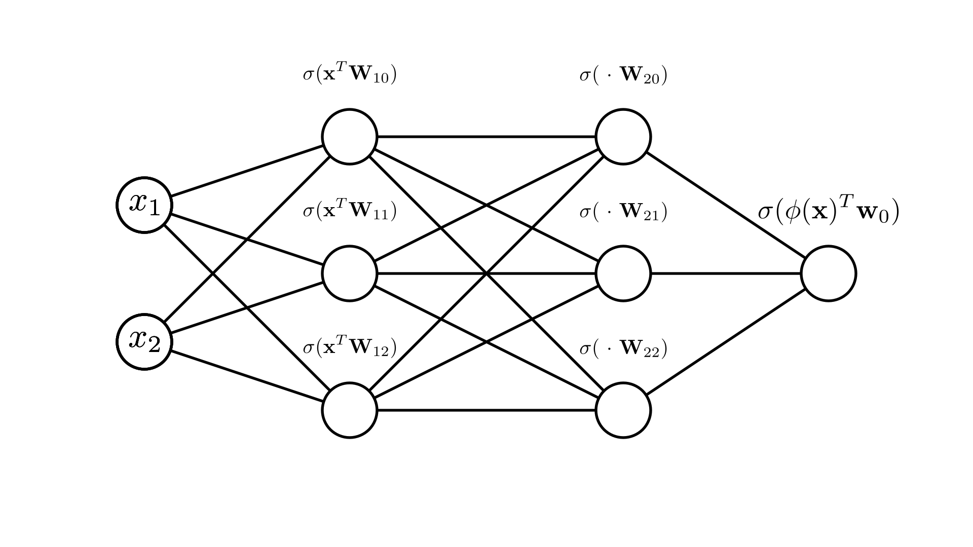
We can see that stacking these transforms allows us to fit even more complicated functions here. Note that we are still not limited to doing this twice! We can fit many layers of transforms:
.svg)
Later on in the semester we’ll talk in more depth about the effect of the number of layers and the number of neurons per layer!
Optimizing neural networks
We can still define a loss function for a neural network in the same way we did with our simpler linear models. The only difference is that now we have more parameters to choose:
\[ \mathbf{Loss}(\mathbf{w}_0,\mathbf{W}_1,...) \]
Let’s look at the logistic regression negative log-likelihood loss for the simple neural network we saw above (for simplicity we’ll just call the network weights \(\mathbf{W}\)). The probability of class 1 is estimated as:
\[ p(y=1\mid \mathbf{x}, \mathbf{w}_0,\mathbf{W})=\sigma(\phi(\mathbf{x})^T \mathbf{w}_0) = \sigma(\sigma(\mathbf{x}^T \mathbf{W}^T) \mathbf{w}_0),\quad \phi(\mathbf{x}) = \begin{bmatrix} \sigma(\mathbf{x}^T \mathbf{W}_{1}) \\ \sigma(\mathbf{x}^T \mathbf{W}_{2}) \\ \sigma(\mathbf{x}^T \mathbf{W}_{3}) \end{bmatrix} \] \[ = \sigma\big(w_{01} \cdot\sigma(x_1 W_{11} + x_2 W_{12}) + w_{02} \cdot\sigma(x_1 W_{21} + x_2 W_{22})+ w_{03} \cdot\sigma(x_1 W_{31} + x_2 W_{32}) \big)\]
Therefore the negative log-likelihood is:
\[ \mathbf{NLL}(\mathbf{w}_0,\mathbf{W}, \mathbf{X}, \mathbf{y}) = -\sum_{i=1}^N \bigg[ y_i\log p(y=1\mid \mathbf{x}, \mathbf{w}_0,\mathbf{W}) + (1-y_i)\log p(y=0\mid \mathbf{x}, \mathbf{w}_0,\mathbf{W}) \bigg] \]
\[ = -\sum_{i=1}^N \log \sigma\big((2y_i-1) \phi(\mathbf{x}_i)^T \mathbf{w}\big) \]
We see that we can write out a full expression for this loss in term of all the inputs and weights. We can even define the gradient of this loss with respect to all the weights:
\[ \nabla_{\mathbf{w}_0} \mathbf{NLL}(\mathbf{w}_0,\mathbf{W}, \mathbf{X}, \mathbf{y}) = \begin{bmatrix} \frac{\partial \mathbf{NLL}}{\partial w_{01}} \\ \frac{\partial \mathbf{NLL}}{\partial w_{02}} \\ \frac{\partial \mathbf{NLL}}{\partial w_{03}} \\ \vdots\end{bmatrix}, \quad \nabla_{\mathbf{W}}\mathbf{NLL}(\mathbf{w}_0,\mathbf{W}, \mathbf{X}, \mathbf{y}) = \begin{bmatrix} \frac{\partial \mathbf{NLL}}{\partial W_{11}} & \frac{\partial \mathbf{NLL}}{\partial W_{12}} & \dots & \frac{\partial \mathbf{NLL}}{\partial W_{1d}} \\ \frac{\partial \mathbf{NLL}}{\partial W_{21}} & \frac{\partial \mathbf{NLL}}{\partial W_{22}} & \dots & \frac{\partial \mathbf{NLL}}{\partial W_{2d}} \\ \vdots & \vdots & \ddots & \vdots \\ \frac{\partial \mathbf{NLL}}{\partial W_{h1}} & \frac{\partial \mathbf{NLL}}{\partial W_{h2}} & \dots & \frac{\partial \mathbf{NLL}}{\partial W_{hd}} \end{bmatrix} \]
Note that as \(\mathbf{W}\) is a matrix, the gradient with respect to \(\mathbf{W}\) is also a matrix! Our gradient descent algorithm can proceed in the same way it did for our linear models, but here we now need to update both sets of parameters:
\[ \mathbf{w}_0^{(k+1)} \longleftarrow \mathbf{w}_0^{(k)} -\alpha \nabla_{\mathbf{w}_0} \mathbf{NLL}(\mathbf{w}_0,\mathbf{W}, \mathbf{X}, \mathbf{y}), \quad \mathbf{W}^{(k+1)} \longleftarrow \mathbf{W}^{(k)} -\alpha \nabla_{\mathbf{W}} \mathbf{NLL}(\mathbf{w}_0,\mathbf{W}, \mathbf{X}, \mathbf{y}) \]
The important question now becomes: how do we compute these gradients?
Automatic Differentiation
In this section we’ll derive algorithms for computing the derivative of any function.
Motivation
We saw above that the NLL for logistic regression with a neural network is:
\[ \mathbf{NLL}(\mathbf{w}_0,\mathbf{W}, \mathbf{X}, \mathbf{y}) = -\sum_{i=1}^N \log \sigma\big((2y_i-1) \phi(\mathbf{x}_i)^T \mathbf{w}\big) \]
If we write this out in terms of the individual values we get:
\[ = -\sum_{i=1}^N \log \sigma\big((2y_i-1)\sigma\big(w_{01} \cdot\sigma(x_1 W_{11} + x_2 W_{12}) + w_{02} \cdot\sigma(x_1 W_{21} + x_2 W_{22})+ w_{03} \cdot\sigma(x_1 W_{31} + x_2 W_{32}) \big)\big) \]
We could use the same approach as usual to find the derivative of this loss with respect to each individual weight parameter, but it would be very tedious and this is only a single-layer network! Things would only get more complicated with more layers. Furthermore if we changed some aspect of the network, like the activation function, we’d have to do it all over again.
Ideally we’d like a programmatic way to compute derivatives. Knowing that we compute derivatives using a fixed set of known rules, this should be possible!
The chain rule revisited
While we often think about the chain rule in terms of functions:
\[ \frac{d}{dx}f(g(x)) = f'(g(x))g'(x) \]
It’s often easier to view it imperatively, in terms of individual values. For example we might say:
\[ b = g(x) \]
\[ a = f(b) \]
In this case we can write the chain rule as:
\[ \frac{da}{dx} = \frac{da}{db}\frac{db}{dx} \]
This corresponds with how we might think about this in code. For example we might have the code:
b = x ** 2
a = log(b)
In this case we have:
\[ a = \log(b), \quad b = x^2 \]
We can compute the derivative of \(a\) with respect to \(x\) using the chain rule as:
\[ \frac{da}{db} = \frac{1}{b}, \quad \frac{db}{dx} = 2x \]
\[ \frac{da}{dx} = \bigg(\frac{1}{b}\bigg)(2x) = \frac{2x}{x^2} = \frac{2}{x} \]
Composing many operations
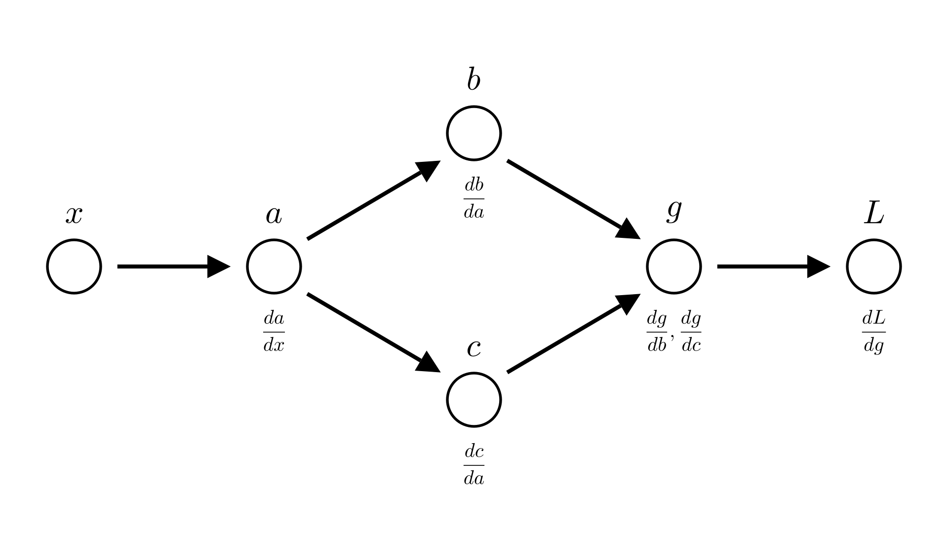
For more complex functions, we might be composing many more operations, but we can break down derivative computations in the same way. For example, if we want the derivative with respect to \(x\) of some simple loss:
\[ L=-\log \sigma\big(w x^2\big) \]
We can break this down into each individual operation that we apply:
\[ a = x^2 \]
\[ b=wa \]
\[ c=\sigma(b) \]
\[ g= \log c \]
\[
L=-g
\]
The chain rule tells us that:
\[
\frac{dL}{dx} = \frac{dL}{dg}\frac{dg}{dc}\frac{dc}{db}\frac{db}{da}\frac{da}{dx}
\]
Since each step is a single operation with a known derivative, we can easily compute every term above! Thus, we begin to see a recipe for computing derivatives programatically. Every time we perform some operation, we will also compute the derivative with respect to the input (we can’t just compute the derivatives because each derivative needs the preceding value, e.g. \(\frac{dg}{dc}=\frac{1}{c}\), so we need to first compute \(c\)).
We can visually look at the chain of computation that we’re performing as a diagram that shows each step and the result.
Manim Community v0.18.1
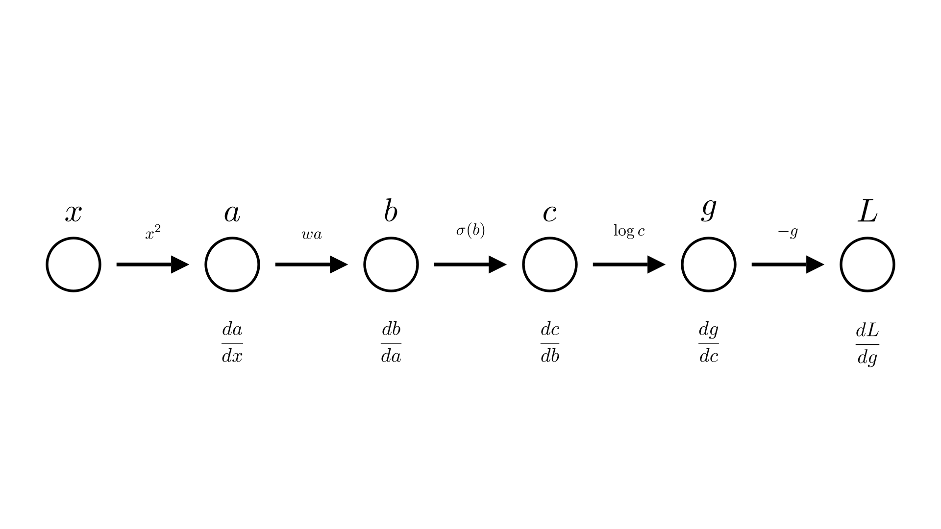
We call this structure the computational graph.
Forward and reverse mode automatic differentiation
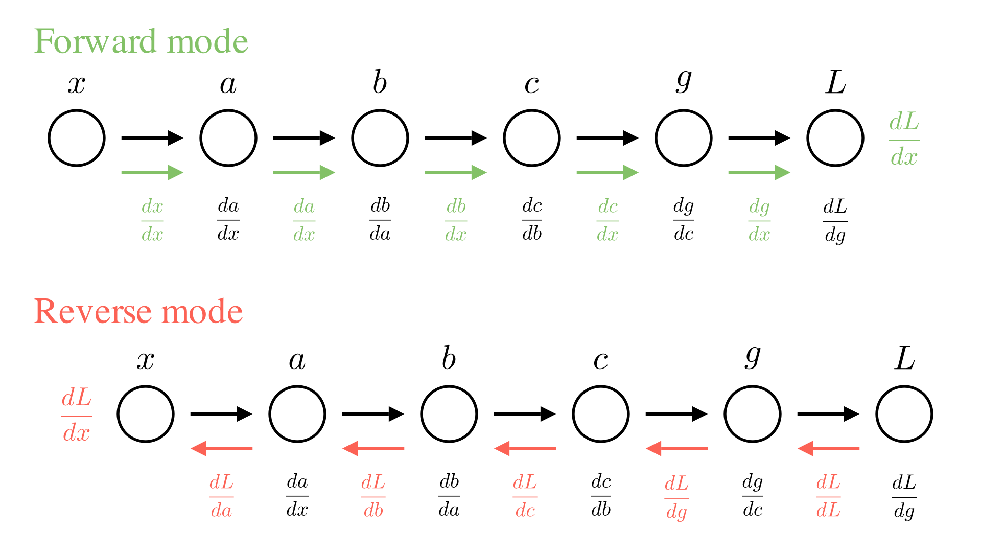
We are not actually interested in all of the intermediate derivatives ( \(\frac{db}{da}, \frac{dc}{db}\) etc.), so it doesn’t make much sense to compute all of them and then multiply them together. Instead, we’d rather just incrementally compute the value we’re interested in \(\frac{dL}{dx}\), as we go.
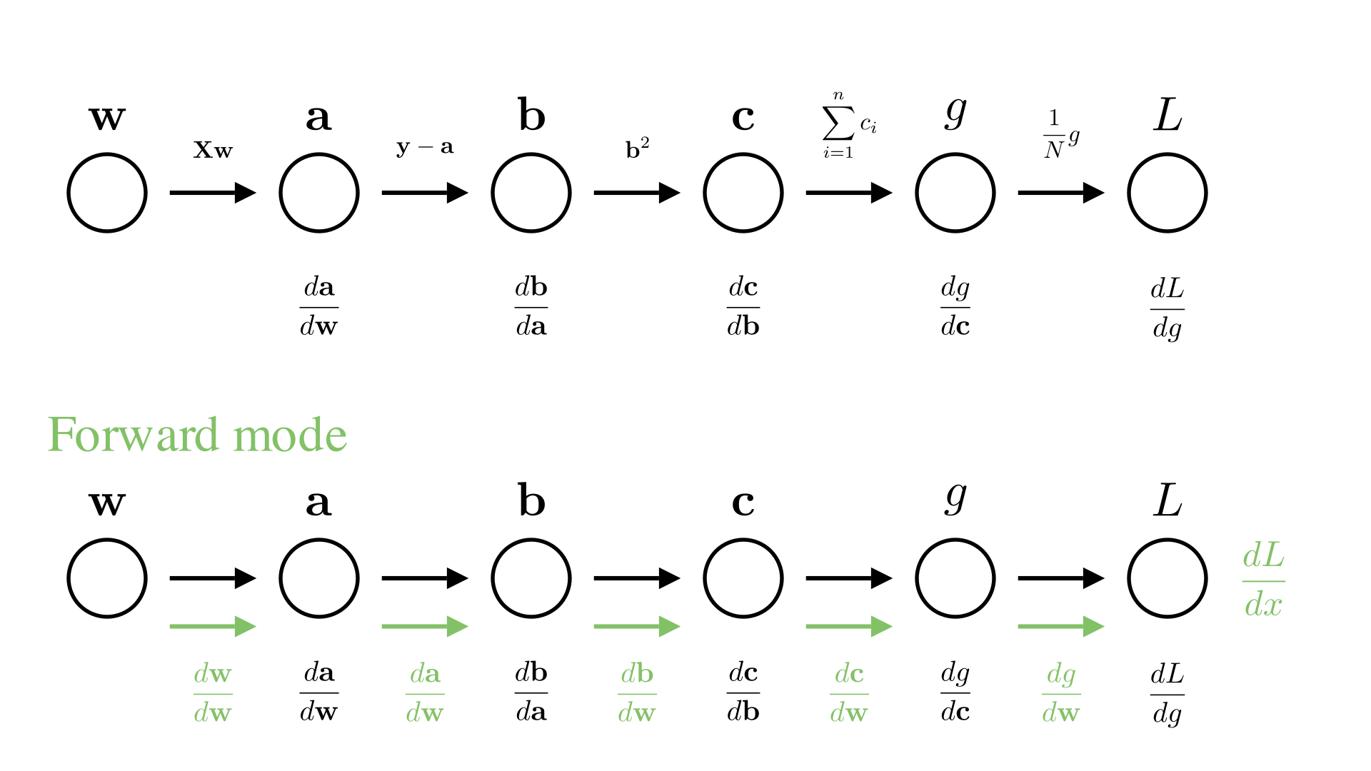
There are 2 ways we could consider doing this. One way is to always keep track of the derivative of the current value with respect to \(x\). So in the diagram above, each time we perform a new operation we will also compute the derivative of the operation and then update our knowledge of the derivative with respect to \(x\). For example for the operation going from \(b\) to \(c\):
\[ c \leftarrow \sigma(b), \quad \frac{dc}{dx} \leftarrow \frac{dc}{db}\cdot\frac{db}{dx} \]
We call this approach forward-mode automatic differentiation.
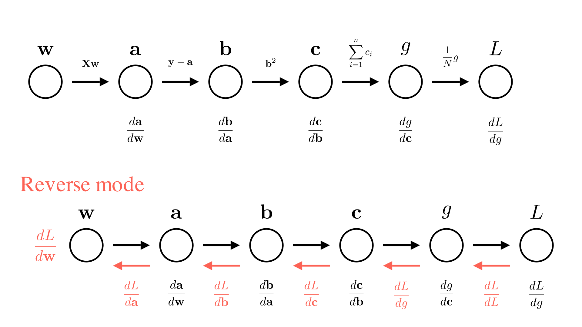
The alternative approach is to work backwards, first compute \(L\) and \(\frac{dL}{dg}\) and then go backwards through the chain updating the derivative of the final output with respect to each input for the \(b\) to \(c\) operation this looks like:
\[ c \leftarrow \sigma(b), \quad \frac{dL}{db} \leftarrow \frac{dc}{db}\cdot\frac{dL}{dc} \]
This means we need to do our computation in 2 passes. First we need to go through the chain of operations to compute \(L\), then we need to go backwards through the chain to compute \(\frac{dL}{dx}\). Note that computing each intermediate derivative requires the a corresponding intermediate value (e.g. \(\frac{dc}{db}\) requires \(b\) to compute). So we need to store all the intermediate values as we go. The approach is called reverse-mode automatic differentiation or more commonly: backpropagation. We can summarize both approaches below:
Manim Community v0.18.1
Automatic differentiation with multiple inputs
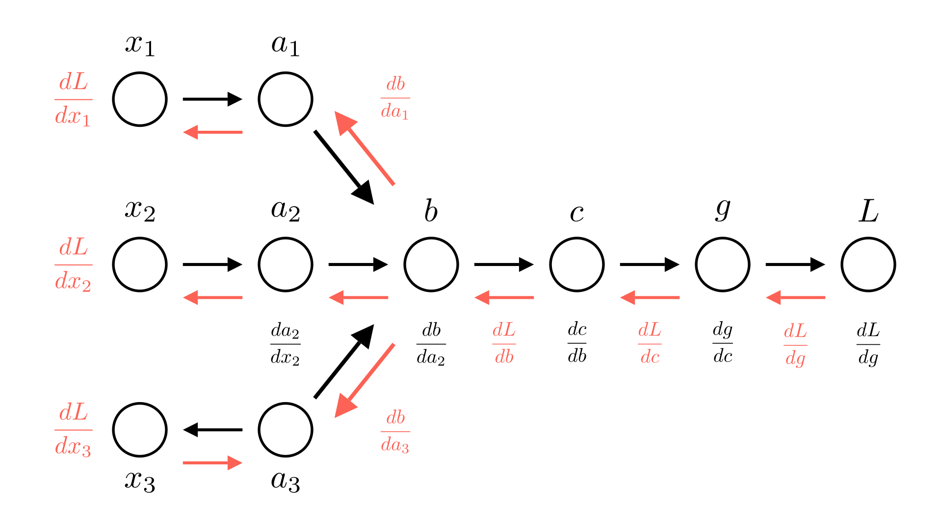
You might wonder why we’d ever use reverse-mode when it seems to require much more complication in keeping track of all the intermediate values. To see why it is useful, lets’s consider the common case where we would like to take derivatives with respect to multiple inputs at the same time. For example we might have an expression like:
\[ -\log \sigma (w_1 x_1+w_2x_2 +w_3x_3) \]
In this case we want to find the gradient:
\[ \frac{dL}{d\mathbf{x}} = \begin{bmatrix}\frac{dL}{dx_1} \\ \frac{dL}{dx_2} \\ \frac{dL}{dx_3} \end{bmatrix} \]
We see that in forward mode, we now need to keep a vector of gradients at many steps if we want to compute the derivative with respect to every input!
Manim Community v0.18.1

In reverse mode, however we only ever need to keep the derivative of the loss with respect to the current value. If we assume that the loss is always a single value, this is much more efficient!
Manim Community v0.18.1
Reusing values
One thing we need to consider is the fact that values can be used in multiple different operations. For example, consider the code below.
def loss(x):
    a = x ** 2
    b = 5 * a
    c = log(a)
    g = b * c
    L = -g
    return L
This corresponds to the following sequence of operations:
\[ a = x^2 \]
\[ b=5a \]
\[ c=\log a \]
\[ g = bc \]
\[ L=-b \]
We see that both \(b\) and \(c\) depend on \(a\). Leading to the following computational graph:
Manim Community v0.18.1
In forward mode this means that we compute 2 different values for \(\frac{dg}{dx}\), one from \(b\) \((\frac{dg}{db}\cdot\frac{db}{dx})\) and one from \(c\) \((\frac{dg}{dc}\cdot\frac{dc}{dx})\).
Manim Community v0.18.1

In reverse mode this means that we compute 2 different values for \(\frac{dL}{da}\), one from \(b\) \((\frac{dL}{db}\cdot\frac{db}{da})\) and one from \(c\) \((\frac{dL}{dc}\cdot\frac{dc}{da})\).
Manim Community v0.18.1

The resolution in both cases is simple! Just add the two terms. So in forward mode:
\[\frac{dg}{dx} = \frac{dg}{db}\cdot \frac{db}{dx} +\frac{dg}{dc}\cdot \frac{dc}{dx}\]
In reverse mode:
\[\frac{dL}{da} = \frac{dL}{db}\cdot \frac{db}{da} + \frac{dL}{dc}\cdot \frac{dc}{da} \]
The forward case for this example is just an application of the product rule:
\[ g =bc \]
\[ \frac{dg}{dx} =\frac{dg}{db}\cdot \frac{db}{dx} +\frac{dg}{dc}\cdot \frac{dc}{dx} = c\cdot \frac{db}{dx} +b \cdot \frac{dc}{dx} \]
For reverse mode we need to expand an rearrange a bit:
\[ \frac{dL}{da} =\frac{dL}{dg}\cdot \frac{dg}{da} \]
\[ \frac{dg}{da} =\frac{dg}{db}\cdot \frac{db}{da} +\frac{dg}{dc}\cdot \frac{dc}{da} \]
\[ \frac{dL}{da} =\frac{dL}{dg}\bigg( \frac{dg}{db}\cdot \frac{db}{da} +\frac{dg}{dc}\cdot \frac{dc}{da} \bigg) \]
\[ =\frac{dL}{dg} \frac{dg}{db} \frac{db}{da} + \frac{dL}{dg}\frac{dg}{dc} \frac{dc}{da} \]
\[ =\frac{dL}{db}\cdot \frac{db}{da} + \frac{dL}{dc}\cdot \frac{dc}{da} \]
This also works for addition:
\[ g =b + c \]
\[ \frac{dg}{dx} =\frac{dg}{db}\cdot \frac{db}{dx} +\frac{dg}{dc}\cdot \frac{dc}{dx} \]
\[ \frac{dg}{db}=1,\ \frac{dg}{dc}=1 \]
\[ \frac{dg}{dx} =\frac{db}{dx} + \frac{dc}{dx} \]
And in general any binary operation! (Division, powers etc.).
Partial and total derivatives
So far we’ve been a bit sloppy in our discussion of derivatives. To see why, let’s consider one more case:
\[ a = x^2 \]
\[ b=5a \]
\[ c = a b \]
\[ L=-c \]
Manim Community v0.18.1
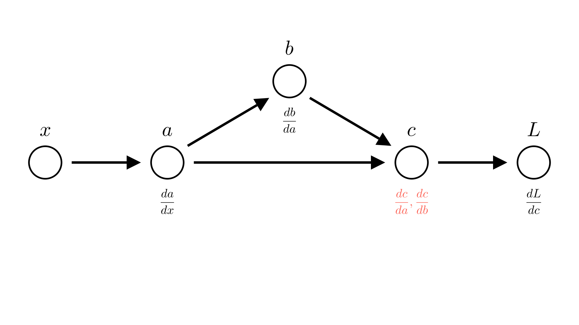
Saying that \(\frac{dc}{da}=b\) isn’t quite correct, because \(b\) also depends on \(a\), really \(\frac{dc}{da} =\frac{dc}{da}+\frac{dc}{db}\frac{db}{da}\). We already account for this in our automatic differentiation though, so we want a way to talk about the derivative of an operation with respect to it’s inputs ignoring how the inputs may depend on each other.
This is where the notion of a partial derivative comes in, the partial derivative of function with respect to an input is the derivative ignoring any dependencies between inputs. We’ve already seen how we denote this:
\[ \frac{\partial c}{\partial a} = b =5a \]
The total derivative is the derivative where we do account for this. In our example:
\[
\frac{dc}{da} =\frac{\partial c}{\partial a}+\frac{\partial c}{\partial b}\frac{\partial b}{\partial a} = 5a + 5a = 10a
\]
In our earlier examples, we typically had partial derivatives equal to total derivatives, so the distinction wasn’t really important. This example shows why it is.
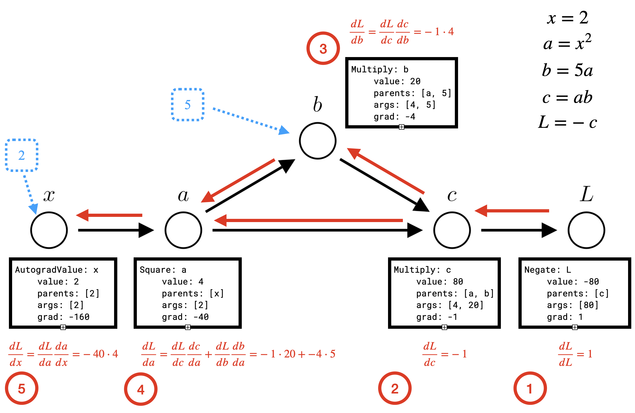
Let’s see our earlier example, but this time we’ll make the distinction between partial and total derivatives explicit
Manim Community v0.18.1
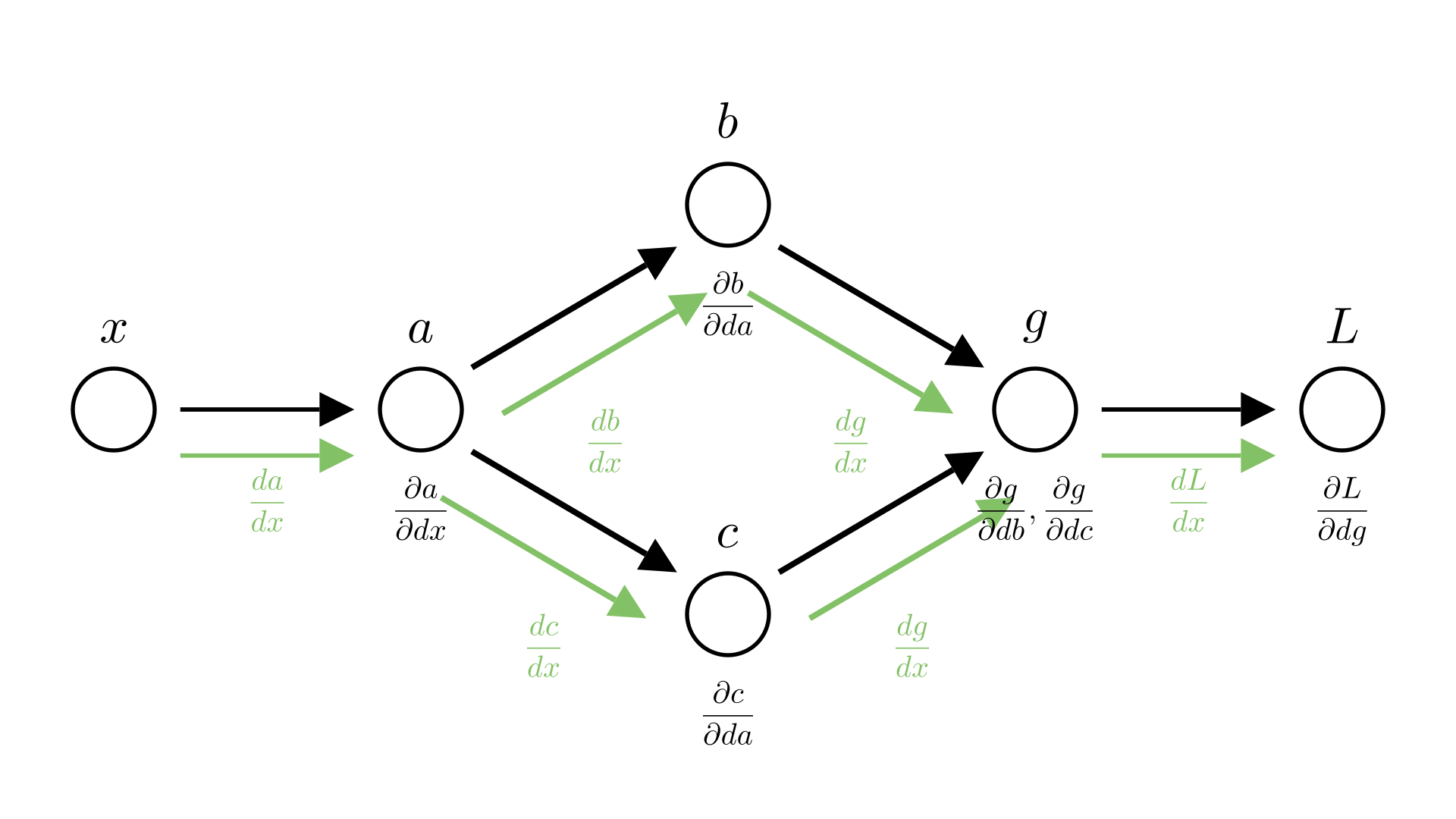
Manim Community v0.18.1
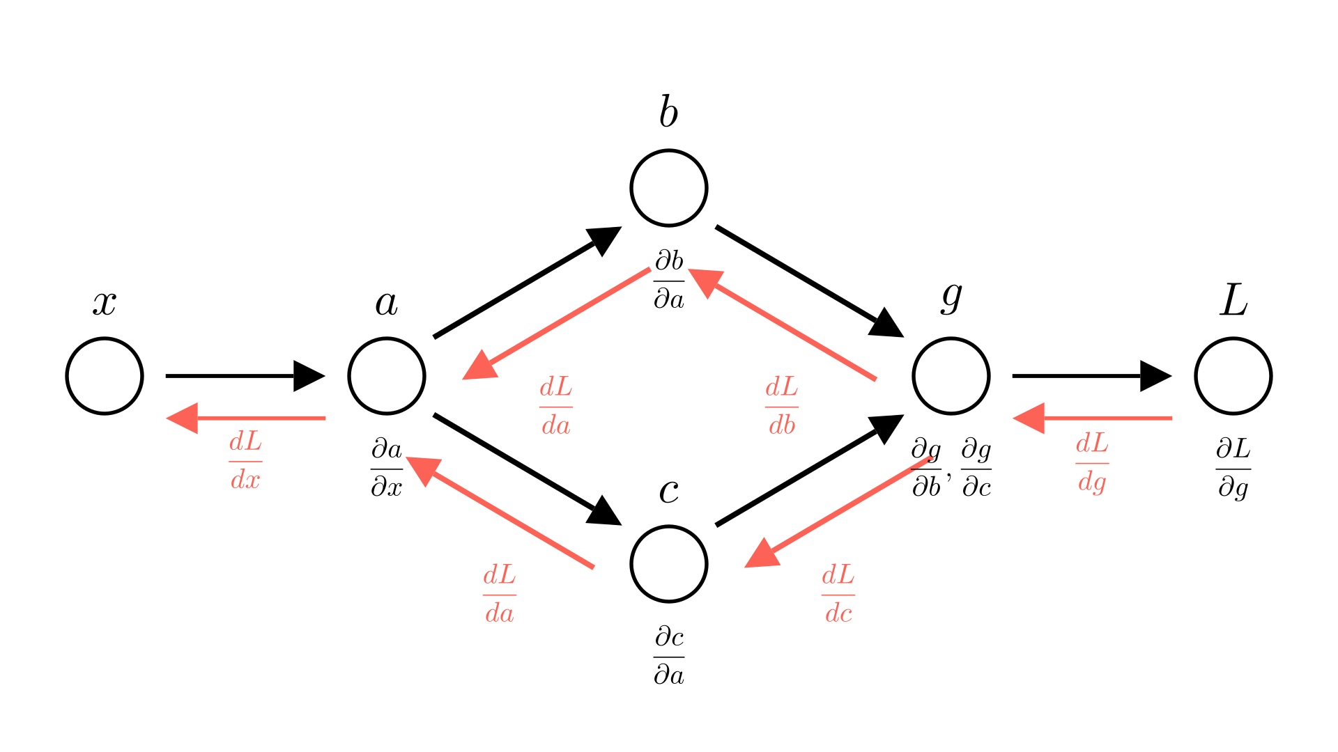
This is also why we specify gradients in terms of partial derivatives! If we’re taking the gradient of a function with respect to multiple inputs, we don’t know where these inputs come from. They might depend on each other! By specifying gradients at partial derivatives, we make it clear that we’re not accounting for that.
Implementing reverse-mode automatic differentiation
We’ll start by developing an automatic differentiation class that uses reverse-mode automatic differentiation, as this is what will be most useful for neural networks.
Recall that for reverse-mode AD to work, everytime we perform an operation on one or more numbers we need to store the result of that operation as well as the parent values (the inputs to the operation). We also need to be able to compute the derivative of that operation. Since for every operation we need to store several pieces of data and several functions, it makes sense to define a class to represent the result of an operation.
For example, if we want to make a class that represents the operation c=a+b our class needs several properties:
value: The value of the operation (c)parents: The parent operations (aandb)grad: The derivative of the final loss with respect toc(\(\frac{dL}{dc}\))func: A function that computes the operation (a+b)grads: A function that computes the derivatives of the operation (\(\frac{dc}{da}\) and \(\frac{dc}{db}\))
For this example, we’ll call our class AutogradValue. This will be the base class for all of our possible operations and represents declaring a variable with a value (a = 5). This is useful because it lets us define values that we might want to find derivatives with respect to.
Let’s see how this will work in practice. If we want to take derivatives we will first define the inputs using AutogradValue.
a = AutogradValue(5)
b = AutogradValue(2)
Then we can perform whatever operations we want on these inputs:
c = a + b
L = log(c)
Each of these operations will produce a new AutogradValue object representing the result of that operation.
Finally we can run the backward pass by running a method backward() (that we will write) on the outout L. This will compute the gradients of L with respect to each input that we defined (\(\frac{dL}{da}\) and \(\frac{dL}{db}\)). Rather than returning these derivatives, the backward() method will update the grad property of a and b, making it easy to access the correct derivative.
L.backward()
dL_da = a.grad
We’ll also be able to compute operations with non-AutogradValue numbers, but obviously won’t be able to compute derivaitives with respect to these values.
s = 4
L = s * a
dL_da = a.grad # Will work because a is an AutogradValue
dL_ds = s.grad # Will give an error because s is not an AutogradValue
Let’s look at one possible implementation for AutogradValue:
class AutogradValue:
    '''
    Base class for automatic differentiation operations.
    Represents variable delcaration. Subclasses will overwrite
    func and grads to define new operations.

    Properties:
        parents (list):  A list of the inputs to the operation,
                         may be AutogradValue or float
        args    (list):  A list of raw values of each
                         input (as floats)
        grad    (float): The derivative of the final loss with
                         respect to this value (dL/da)
        value   (float): The value of the result of this operation
    '''

    def __init__(self, *args):
        self.parents = list(args)
        self.args = [arg.value if isinstance(arg, AutogradValue)
                     else arg
                     for arg in self.parents]
        self.grad = 0.
        self.value = self.forward_pass()

    def forward_pass(self):
        # Calls func to compute the value of this operation
        return self.func(*self.args)
For convenience, in this implementation we’ve also defined a property args which simply stores the value of each parent. Note that we can also allow parents to be either be AutogradValue or a primitive data type like float. This will allow us to do things like multiply an AutogradValue variable with a float, e.g. a * 5.
The forward_pass function computes the actual value of the node given it’s parents. This will depend on what kind of operation we’re doing (addition, subtraction, multiplication, etc.), so we’ll define a func method that we can override that does the actual calculation. In the base case we’ll just directly assign the value:
class AutogradValue:
    def func(self, input):
        '''
        Compute the value of the operation given the inputs.
        For declaring a variable, this is just the identity
        function (return the input).

        Args:
            input (float): The input to the operation
        Returns:
            value (float): The result of the operation
        '''
        return input
In subclasses we’ll override func:
class _square(AutogradValue):
    # Square operator (a ** 2)
    def func(self, a):
        return a ** 2

class _mul(AutogradValue):
    # Multiply operator (a * b)
    def func(self, a, b):
        return a * b
Let’s consider what the computational graph will look like for the following code:
x = AutogradValue(2)
a = x ** 2
b = 5 * a
c = b * a
L = -c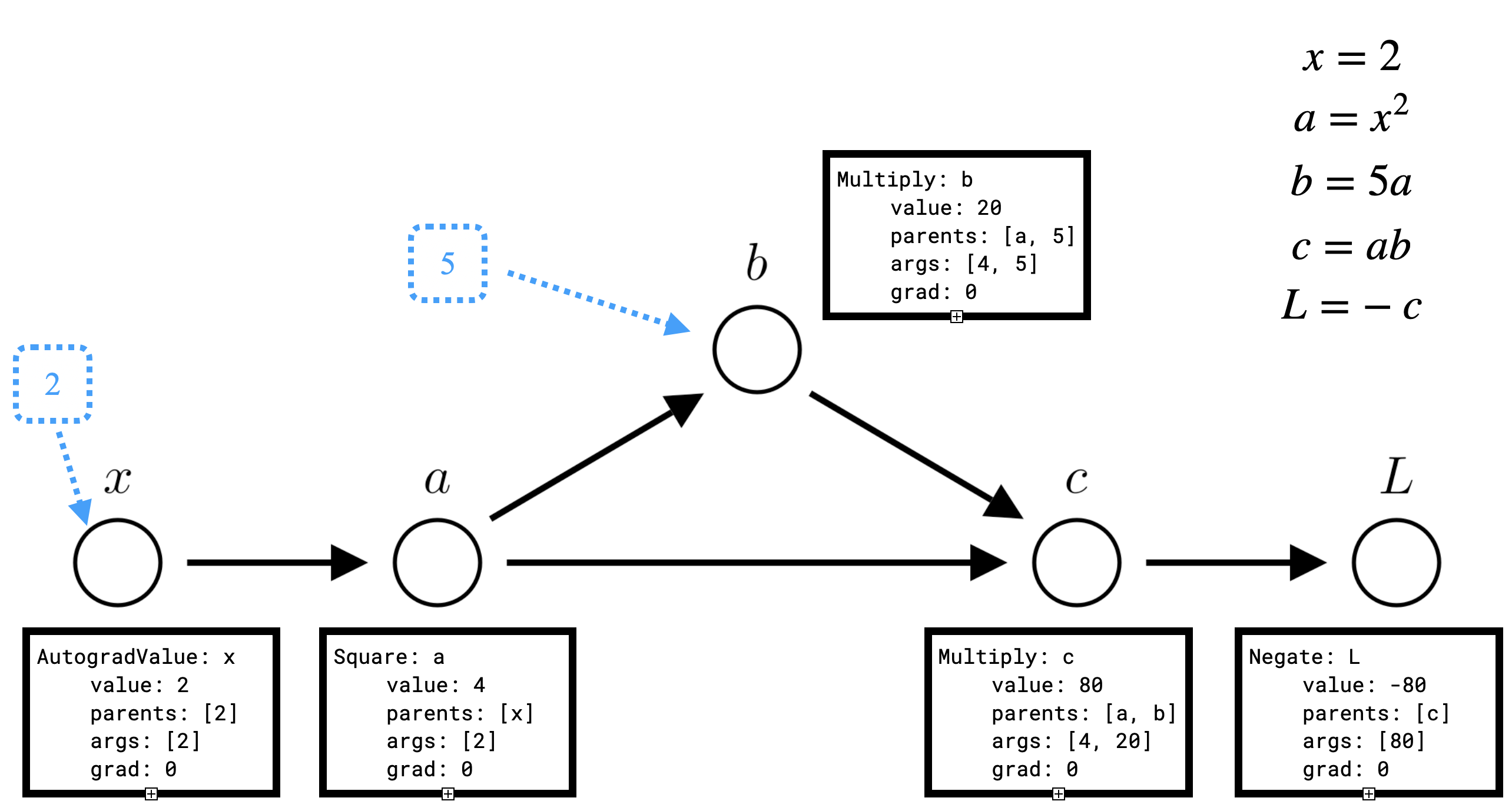
Here the blue nodes represent constants (of type float), while the black nodes are AutogradValue objects. We see that every AutogradValue is populated with the value, parents and args, but that after this first pass grad is still 0 for each object, so we have not computed \(\frac{dL}{dx}\). To do so, we need to run the backward pass by calling L.backward().
L.backward()
print('dL_dx', x.grad)
In the backward pass, each node needs to update the grad property of its parents.
So first \(L\) needs to update the grad property for \(c\), which represents \(\frac{dL}{dc}\). Then \(c\) is able to update the grad property of \(a\) and \(b\) (\(\frac{dL}{da}\) and \(\frac{dL}{db}\)).
Note that the order we perform these updates matters! \(\frac{dL}{da}\) will not be correct until both \(b\) and \(c\) have updated \(a\), thus \(a\) cannot perform the update to \(\frac{dL}{dx}\) until both \(b\) and \(c\) have updated \(a\).
For each operation, we see that we also need to be able to compute the appropriate local derivatives of the value with respect to each input. For instance \(a\) needs to be able to compute \(\frac{da}{dx}\) , \(c\) needs to be able to compute \(\frac{dc}{da}\) and \(\frac{dc}{db}\). We will definite another method grads that can compute these values for a given operation and override it for each subclass. Since grads might need to compute multiple derivatives (as for multiplication or addition) we’ll have it return a tuple.
class AutogradValue:
        def grads(self, *args):
        '''
        Compute the derivative of the operation with respect to each input.
        In the base case the derivative of the identity function is just 1. (da/da = 1).

        Args:
            input (float): The input to the operation
        Returns:
            grads (tuple): The derivative of the operation with respect to each input
                            Here there is only a single input, so we return a length-1 tuple.
        '''
        return (1,)

class _square(AutogradValue):
    # Square operator (a ** 2)
    def grads(self, a):
        return (2 * a,)

class _mul(AutogradValue):
    # Multiply operator (a * b)
    def grads(self, a, b):
        return (b, a)
With this in hand we can write a function that performs the backward update for a given operation. We’ll call this method backward_pass.
Computational graphs of vectors
As we’ve seen, in the context of neural networks we typically perform operations on large collections of values such as vectors. For example, we might perform an element-wise square on a large vector:
x = np.ones((500,))
a = x ** 2
In this case we are performing 500 individual square operations, so our computational graph would look like:
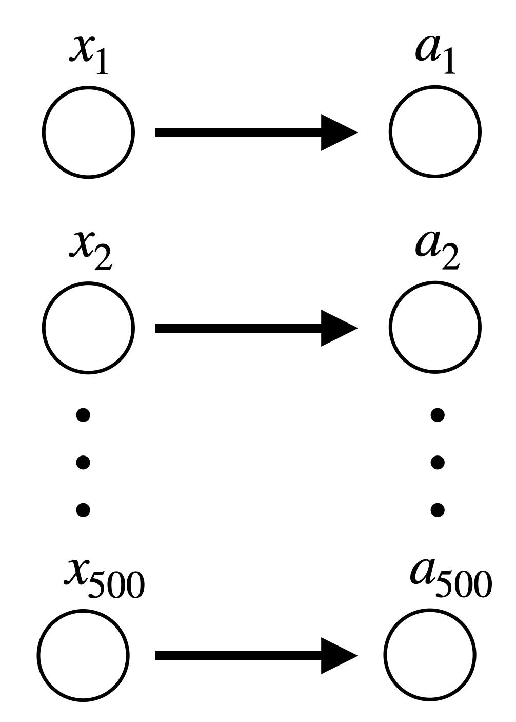
Remember for our automatic differentiation implementation we would need an object for each of these values.
x = np.array([AutogradValue(1), AutogradValue(1), ...])
a = x ** 2
Each of these object introduces some overhead as each object needs to be constructed individually and needs to store not just the value and gradients, but also the parents. Furthermore our backward pass needs to determine the order of nodes to visit. For a large neural network, having a node for every single value would be computationally very complex.
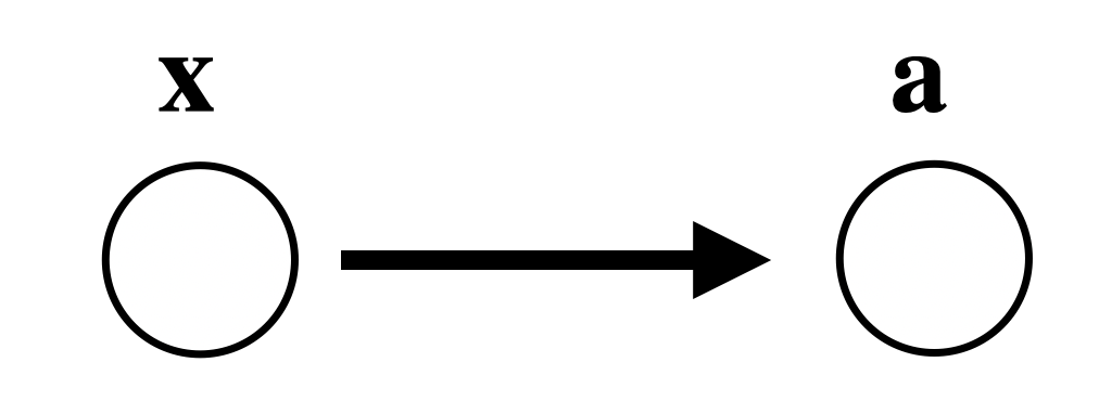
Since we’re performing the same operation on each entry of the vector, there’s really no need to have a separate node for each entry. Therefore we might instead prefer each node in our computational graph to represent a vector or matrix and for our operations to correspond to vector or matrix operations:
x = AutogradValue(np.ones((500,)))
a = x ** 2
In this case the computational graph for this operation would be:
Our derivative calculations can similarly be performed as element-wise operations:
\[ \begin{bmatrix} \frac{da_1}{dx_1} \\ \frac{da_2}{dx_2} \\ \vdots \\ \frac{da_{500}}{dx_{500}} \end{bmatrix} = \begin{bmatrix} 2x_1 \\ 2x_2 \\ \vdots \\ 2x_{500} \end{bmatrix} = 2\mathbf{x} \]
So in fact, for this case, we don’t actually need to change our AutogradValue implementation for square at all!
class _square(AutogradValue):
    # Square operator (a ** 2)
    def func(self, a):
        return a ** 2

    # Returns a vector of the element-wise derivatives!
    def grads(self, a):
        return (a ** 2,)
Automatic differentiation for linear regression
Let’s take a look at a concrete example how reverse-mode automatic differentiation with vectors would work. Specifically let’s look at taking the gradient of the mean squared error loss we used for linear regression.
\[ L = \frac{1}{N}\sum_{i=1}^N (y_i - \mathbf{x}_i^T\mathbf{w})^2 = \frac{1}{N}\sum_{i=1}^N (\mathbf{y} - \mathbf{X}\mathbf{w})_i^2 \]
Here the right-hand side of the expression corresponds to how we might write this formula using numpy:
se = (y - np.dot(X, w)) ** 2
mse = np.sum(se) / X.shape[0]
We are interested in the gradient with respect to \(\mathbf{w}\), or \(\frac{dL}{d\mathbf{w}}\) for optimizing our model. Let’s start by looking at the simplest sequence of operations:
\[ \mathbf{a} = \mathbf{X}\mathbf{w} \]
\[ \mathbf{b} = \mathbf{y} - \mathbf{a} \]
\[ \mathbf{c} = \mathbf{b}^2 \]
\[ g = \sum_{i=1}^N c_i \]
\[ L = \frac{1}{N}g \]
We can setup our computational graph and reverse mode algorithm exactly as we did before, only in this case some of the operations will be on vectors! (\(g\) and \(L\) are still scalars, but \(\mathbf{w}\), \(\mathbf{a}\), \(\mathbf{b}\) and \(\mathbf{c}\) are vectors)
Manim Community v0.18.1

Let’s walk through the computation of \(\frac{dL}{d\mathbf{w}}\).
Computing \(\frac{dL}{dg}\): The first step in the backward pass is straightforward:
\[ \frac{dL}{dg} = \frac{1}{N} \]
Computing \(\frac{dL}{d\mathbf{c}}\):
\[ \frac{dL}{d\mathbf{c}}= \frac{dL}{dg}\frac{dg}{d\mathbf{c}} \]
Since \(\mathbf{c}\) is a vector, \(\frac{dg}{d\mathbf{c}}\) and \(\frac{dL}{d\mathbf{c}}\) must be vectors of the derivative of \(L\) or \(g\) with respect to each entry of \(\mathbf{c}\). In other words \(\frac{dg}{d\mathbf{c}}\) and \(\frac{dL}{d\mathbf{c}}\) are gradients!
\[ \frac{dL}{d\mathbf{c}}= \begin{bmatrix} \frac{dL}{dc_1} \\ \frac{dL}{dc_2} \\ \vdots \\ \frac{dL}{dc_N} \end{bmatrix} = \frac{dL}{dg} \begin{bmatrix} \frac{dg}{dc_1} \\ \frac{dg}{dc_2} \\ \vdots \\ \frac{dg}{dc_N} \end{bmatrix} = \frac{dL}{dg}\frac{dg}{d\mathbf{c}} \]
We know that the derivative of a sum with respect to a single element is \(1\), as in: \(\frac{d}{dc_1}(c_1+c_2)=1\), so it follows that the gradient of our summation is simply a vector of 1s.
\[
\frac{dg}{d\mathbf{c}} =\begin{bmatrix} 1 \\ 1 \\ \vdots \\ 1 \end{bmatrix}, \quad \frac{dL}{d\mathbf{c}} =\begin{bmatrix} 1 \\ 1 \\ \vdots \\ 1 \end{bmatrix}\frac{1}{N} = \begin{bmatrix} \frac{1}{N} \\ \frac{1}{N} \\ \vdots \\ \frac{1}{N} \end{bmatrix}
\]
Computing \(\frac{dL}{d\mathbf{b}}\):
Since \(\mathbf{b}^2\) is an element-wise operation \((c_i=b_i^2)\) we know that:
\[ \frac{dL}{db_i}=\frac{dL}{dc_i}\frac{dc_i}{db_i} = \frac{1}{N}(2b_i) \]
Therefore:
\[ \frac{dL}{d\mathbf{b}} = \begin{bmatrix} \frac{dL}{dc_1}\frac{dc_1}{db_1} \\ \frac{dL}{dc_2}\frac{dc_2}{db_2} \\ \vdots \\ \frac{dL}{dc_N}\frac{dc_N}{db_N} \end{bmatrix} = \begin{bmatrix} \frac{2}{N}b_1 \\ \frac{2}{N}b_2 \\ \vdots \\ \frac{2}{N}b_N \end{bmatrix} \]
Computing \(\frac{dL}{d\mathbf{a}}\):
Since \(\mathbf{y}-\mathbf{a}\) is also an element-wise operation \((b_i=y_i-a_i)\) we similarly see that:
\[ \frac{dL}{da_i}=\frac{dL}{db_i}\frac{db_i}{da_i} = \frac{2b_i}{N}(-1) \]
\[ \frac{dL}{d\mathbf{a}} = \begin{bmatrix} \frac{dL}{db_1}\frac{db_1}{da_1} \\ \frac{dL}{dc_2}\frac{db_2}{da_2} \\ \vdots \\ \frac{dL}{dc_N}\frac{db_N}{da_N} \end{bmatrix} = \begin{bmatrix} \frac{-2}{N}b_1 \\ \frac{-2}{N}b_2 \\ \vdots \\ \frac{-2}{N}b_N \end{bmatrix} \]
Computing \(\frac{dL}{d\mathbf{w}}\):
This last calculation is less straightforward. \(\mathbf{X}\mathbf{w}\) is not an element-wise operation, so we can’t just apply the chain rule element-wise. We need a new approach! Let’s break down the general problem that we see here.
Vector-valued functions
A vector-valued function is a function that takes in a vector and returns a vector:
\[ \mathbf{y} = f(\mathbf{x}), \quad f: \mathbb{R}^n\rightarrow\mathbb{R}^m \]
For example the matrix-vector product we’ve just seen is a simple vector-valued function:
\[ f(\mathbf{w}) =\mathbf{X}\mathbf{w} \]
If \(\mathbf{X}\) is an \((N\times d)\) matrix and \(\mathbf{w}\) is a length- \(d\) vector, then \(f(\mathbf{w})=\mathbf{X}\mathbf{w}\) is a mapping \(\mathbb{R}^d\rightarrow \mathbb{R}^N\)
Jacobians
A the Jacobian \((\mathbf{J})\) of a vector-valued function is the matrix of partial derivatives of every output with respect to every input. We can think of it as an extension of the gradient for vector-valued functions. If we have a vector-valued function \(f\) and \(\mathbf{a}\) is the result of applying \(f\) to \(\mathbf{w}\):
\[ \mathbf{a}=f(\mathbf{w}), \quad f:\mathbb{R}^d\rightarrow \mathbb{R}^N \]
The corresponding Jacobian is:
\[\frac{d\mathbf{a}}{d\mathbf{w}} = \begin{bmatrix} \frac{\partial a_1}{\partial w_1} & \frac{\partial a_1}{\partial w_2}& \dots& \frac{\partial a_1}{\partial w_d} \\ \frac{\partial a_2}{\partial w_1} & \frac{\partial a_2}{\partial w_2}& \dots& \frac{\partial a_2}{\partial w_d} \\ \vdots & \vdots & \ddots & \vdots \\ \frac{\partial a_N}{\partial w_1} & \frac{\partial a_N}{\partial w_2}& \dots& \frac{\partial a_N}{\partial w_d} \\ \end{bmatrix}\]
In general:
\[ \bigg(\frac{d\mathbf{a}}{d\mathbf{w}}\bigg)_{ij} = \frac{\partial a_i}{\partial w_j} \]
Let’s consider the Jacobian of a matrix-vector product:
\[ \mathbf{a} = \mathbf{X}\mathbf{w} \]
We can find each entry in the Jacobian by taking the corresponding partial derivative.
\[ a_i =\sum_{j=1}^d X_{ij}w_j, \quad \frac{\partial a_i}{\partial w_j}=X_{ij} \]
In this case we see that the Jacobian is just \(\mathbf{X}\)!
Vector-Jacobian products
Let’s return to our linear regression example:
Manim Community v0.18.1
We see that \(\frac{d\mathbf{a}}{d\mathbf{w}}\) is actually a Jacobian that we now know how to compute, so the remaining question is how to combine it with \(\frac{dL}{d\mathbf{a}}\) in order to get the gradient we’re looking for \(\frac{dL}{d\mathbf{w}}\)? The answer turns out to be simple: use the vector-matrix product:
\[ \frac{dL}{d\mathbf{w}} = \frac{dL}{d\mathbf{a}}^T\frac{d\mathbf{a}}{d\mathbf{w}} \]
We might be curious why this is the right thing to do as opposed to a matrix-vector product or some other function. To see why, let’s consider what an entry of our final gradient \(\frac{dL}{d\mathbf{w}}\) should be. We’ve previously seen that when a value is use by more than one child operation, we need to sum the contribution of each child to the total derivative. So in this case, for a given entry of \(\mathbf{w}\) we need to sum the gradient contribution from every element of \(\mathbf{a}\):
\[ \frac{dL}{dw_j} = \frac{dL}{da_1} \frac{da_1}{dw_j}+\frac{dL}{da_2} \frac{da_2}{dw_j}+...\frac{dL}{da_N} \frac{da_N}{dw_j} = \sum_{i=1}^N \frac{dL}{da_i} \frac{da_i}{dw_j} \]
Which we can see is equivalent to an entry in the vector matrix product:
\[ \frac{dL}{d\mathbf{w}} = \begin{bmatrix} \frac{dL}{da_1} & \frac{dL}{da_2} & ... & \frac{dL}{da_N} \end{bmatrix}\begin{bmatrix} \frac{\partial a_1}{\partial w_1} & \frac{\partial a_1}{\partial w_2}& \dots& \frac{\partial a_1}{\partial w_d} \\ \frac{\partial a_2}{\partial w_1} & \frac{\partial a_2}{\partial w_2}& \dots& \frac{\partial a_2}{\partial w_d} \\ \vdots & \vdots & \ddots & \vdots \\ \frac{\partial a_N}{\partial w_1} & \frac{\partial a_N}{\partial w_2}& \dots& \frac{\partial a_N}{\partial w_d} \\ \end{bmatrix} = \frac{dL}{d\mathbf{a}}^T\frac{d\mathbf{a}}{d\mathbf{w}} \]
We call this a vector-Jacobian product or VJP for short. We see that because it’s simply derived from our basic gradient rules, it’s valid for any vector-valued operation, as long as we can compute the Jacobian! We can use this to perform the final step in the backward pass for the MSE.
Computing \(\frac{dL}{d\mathbf{w}}\):
From our vector-Jacobian product rule we know that:
\[ \frac{dL}{d\mathbf{w}} = \frac{dL}{d\mathbf{a}}^T\frac{d\mathbf{a}}{d\mathbf{w}}= \frac{-2}{N}\mathbf{b}^T\mathbf{X} \]
If we substitute back in \(\mathbf{b}=\mathbf{y}-\mathbf{X}\mathbf{w}\) we see that this is equivalent to the gradient we derived in a previous class!
\[ \frac{dL}{d\mathbf{w}} = \frac{-2}{N}(\mathbf{y}-\mathbf{X}\mathbf{w})^T\mathbf{X} \]
VJPs for element-wise operations
It’s worth noting that element-wise operations are still vector-valued functions.
\[ \mathbf{c}=\mathbf{b}^2, \quad \mathbb{R}^n\rightarrow\mathbb{R}^n \]
So why didn’t we need to do a vector-Jaobian product for that operation? The answer is that we did, just implicitly! If we consider the Jacobian for this operation we see that because each entry of \(\mathbf{c}\) only depends on the corresponding entry of \(\mathbf{b}\), the Jacobian for this operation is \(0\) everywhere except the main diagonal:
\[ \frac{d\mathbf{c}}{d\mathbf{b}} = \begin{bmatrix} \frac{\partial c_1}{\partial b_1} & 0 & \dots& 0 \\ 0 & \frac{\partial c_2}{\partial b_2}& \dots& 0\\ \vdots & \vdots & \ddots & \vdots \\ 0& 0& \dots& \frac{\partial c_N}{\partial b_d} \\ \end{bmatrix} \]
This means that we can write the vector-Jacobian product as we did before:
\[ \frac{dL}{d\mathbf{c}}\frac{d\mathbf{c}}{d\mathbf{b}}=\begin{bmatrix} \frac{dL}{dc_1}\frac{dc_1}{db_1} \\ \frac{dL}{dc_2}\frac{dc_2}{db_2} \\ \vdots \\ \frac{dL}{dc_N}\frac{dc_N}{db_N} \end{bmatrix} \]
This is a big computational savings over explicitly constructing the full Jacobian and performing a vector-matrix multiplication.
VJPs for matrices
So far we’ve seen VJPs with respect to vectors. What if in the formulation above, we were to take the derivative with respect to \(\mathbf{X}\) instead of \(\mathbf{w}\)?
\[ \mathbf{a}=\mathbf{X}\mathbf{w},\quad \frac{d\mathbf{a}}{d\mathbf{X}} \]
In this case \(\mathbf{X}\) is an \(N\times d\) matrix, so if we were to consider all the partial derivatives making up the Jacobian \(\frac{d\mathbf{a}}{d\mathbf{X}}\) there would be \(N\times N\times d\) values, while the gradient \(\frac{dL}{d\mathbf{X}}\) is itself an \(N\times d\) matrix of the derivative of \(L\) with respect to each value of \(\mathbf{X}\).
Let’s look at how we can formulate the vector-Jacobian product:
\[ \frac{dL}{d\mathbf{X}} = \frac{dL}{d\mathbf{a}}^T\frac{d\mathbf{a}}{d\mathbf{X}} \]
We know that for a given entry of \(\frac{dL}{d\mathbf{X}}\), we can again compute the derivative by summing the contribution from each child, in this case every entry of \(\mathbf{a}\)
\[ \frac{dL}{dX_{jk}} = \sum_{i=1}^N \frac{\partial L}{\partial a_{i}} \frac{\partial a_i}{\partial X_{jk}} \]
This suggests that we can compute the VJP by flattening the Jacobian from an \(N\times N \times d\) structure into a \(N \times Nd\) matrix. Therefore performing the vector-matrix product will give us a length \(Nd\) vector with the appropriate values for us to reshape into our \(N \times d\) Jacobian \(\frac{dL}{d\mathbf{X}}\).
In code this could look like:
dL_da, da_dx  # The computed gradients/jacobians
da_dx = da_dx.reshape((da_dx.shape[0], -1))
dL_dx = np.dot(dL_da, da_dx)
dL_dx = dL_dx.reshape(x.shape)
Let’s return to our example:
\[\mathbf{a}=\mathbf{X}\mathbf{w}\]
Do we need to instantiate the full Jacobian here? No! In our original operation:
\[ a_i = \sum_{k=1}^d X_{ik}w_k \]
Thus \(\frac{\partial a_i}{\partial X_{jk}}\) is only nonzero when \(j=i\). Taking the derivative we get:
\[ \frac{\partial a_i}{\partial X_{jk}} = \frac{\partial}{\partial X_{jk}}\sum_{k=1}^d X_{ik}w_k = \mathbb{I}(i=j)w_k \]
We can therefore write the vector-Jacobian product as:
\[ \frac{\partial L}{\partial X_{ik}}=\frac{\partial L}{\partial a_i}\frac{\partial a_i}{\partial X_{ik}} = \frac{\partial L}{\partial a_i}w_k \]
In code we could write this as:
w_mat = w.reshape((1, -1)) # reshape w to 1 x d
dL_da_mat = dL_da.reshape((-1, 1)) # reshape dL_da to N x 1
dL_dx = w_mat * dL_da_mat # dL_dx becomes N x d, entry ik = dL_da_i * w_k
Forward mode AD with vectors
What about forward mode for our linear regression example?
\[ \mathbf{a} = \mathbf{X}\mathbf{w} \]
\[ \mathbf{b} = \mathbf{y} - \mathbf{a} \]
\[ \mathbf{c} = \mathbf{b}^2 \]
\[ g = \sum_{i=1}^N c_i \]
\[ L = \frac{1}{N}g \]
Manim Community v0.18.1
As we’ve seen \(\frac{d\mathbf{a}}{d\mathbf{w}}\) is an \(N\times d\) Jacobian matrix. After computing this, the next step will be to compute:
\[\frac{d\mathbf{b}}{d\mathbf{w}}=\frac{d\mathbf{b}}{d\mathbf{a}}\frac{d\mathbf{a}}{d\mathbf{w}}\]
Here we are multiplying the \(N\times N\) Jacobian \(\frac{d\mathbf{b}}{d\mathbf{a}}\) with the \(N\times d\) gradient \(\frac{d\mathbf{a}}{d\mathbf{w}}\) to get the \(N\times d\) gradient \(\frac{d\mathbf{b}}{d\mathbf{w}}\). We can again verify that this is the correct computation by checking an individual element of \(\frac{d\mathbf{b}}{d\mathbf{w}}\):
\[ \frac{db_i}{dw_j}=\sum_{k=1}^N \frac{db_i}{da_k}\frac{da_k}{dw_j} \]
We call this operation a Jacobian-vector product or JVP.