Homework 1: Introduction to Numpy (solutions)

Python setup

# Run me first!
import numpy as np
import matplotlib.pyplot as plt
import seaborn as sns
sns.set_style('darkgrid')

Part 1: Numpy basics

As discussed in class, a square matrix \(A\) defines a linear mapping: \(\mathbb{R}^n\rightarrow \mathbb{R}^n\). Given a vector \(\textbf{x}\), we can find the corresponding output of this mapping \(\textbf{b}\) using matrix-vector multiplication: \(\textbf{b}=A \textbf{x}\). We can write an example matrix-multiplication using matrix notation as:

\[\begin{bmatrix} 4 & -3 & 2 \\ 6 & 5 & 1 \\ -4 & -1 & 2 \end{bmatrix} \cdot \begin{bmatrix} 1 \\ -2 \\ 1 \end{bmatrix} = \begin{bmatrix} ? \\ ? \\ ? \end{bmatrix} \]

Q1

Perform this matrix-vector multiplication by hand and write the answer in the cell below.

Answer

Performing the matrix-vector multiplication by hand:

\[\begin{bmatrix} 4 & -3 & 2 \\ 6 & 5 & 1 \\ -4 & -1 & 2 \end{bmatrix} \cdot \begin{bmatrix} 1 \\ -2 \\ 1 \end{bmatrix} = \begin{bmatrix} 4(1) + (-3)(-2) + 2(1) \\ 6(1) + 5(-2) + 1(1) \\ -4(1) + (-1)(-2) + 2(1) \end{bmatrix} = \begin{bmatrix} 4 + 6 + 2 \\ 6 - 10 + 1 \\ -4 + 2 + 2 \end{bmatrix} = \begin{bmatrix} 12 \\ -3 \\ 0 \end{bmatrix} \]

Q2

In the code cell below, create the matrix \(A\) and the vector \(\textbf{x}\) shown above, using Numpy. Then use the np.dot function to find the output of the mapping \(\textbf{b} = A\textbf{x}\). Verify that the answer matches what you derived above.

Answer

# Fill answers here
A = np.array([[4, -3, 2],
              [6, 5, 1],
              [-4, -1, 2]
              ])
x = np.array([1, -2, 1])
b = np.dot(A, x)

print(b)

[12 -3  0]

Often we will have access to the transformed vector \(\textbf{b}\) and need to find the orginal vector \(\textbf{x}\). To do this we need to solve the system of linear equations \(A\textbf{x}=\textbf{b}\) for \(\textbf{x}\). \[\begin{bmatrix} 4 & -3 & 2 \\ 6 & 5 & 1 \\ -4 & -1 & 2 \end{bmatrix} \cdot \begin{bmatrix} ? \\ ? \\ ? \end{bmatrix} = \begin{bmatrix} 2 \\ -1 \\ 3 \end{bmatrix} \]

Q3

Find the missing \(\textbf{x}\) in the equation above using the np.linalg.solve function and verify that \(A\textbf{x}=\textbf{b}\).

Answer

b = np.array([2, -1, 3])
x = np.linalg.solve(A, b)
print(b, np.dot(A, x))

[ 2 -1  3] [ 2. -1.  3.]

In linear algebra you may have learned how to solve a system of linear equations using Gaussian elimination. Here we will implement an alternative approach known as Richardson iteration. In this method we start with an inital guess for the solution: \(\textbf{x}^{(0)}\), then we will iteratively update this guess until the solution is reached. Given a matrix \(A\), a target \(\textbf{b}\) and a current guess \(\textbf{x}^{(k)}\), we can compute the Richardson update as:

\[\textbf{x}^{(k+1)} \leftarrow \textbf{x}^{(k)} + \omega \left(\textbf{b} - A\textbf{x}^{(k)}\right)\]

Here \(\omega\) is a constant that we can choose to adjust the algorithm. We will set \(\omega = 0.1\).

Q4

Fill in the Richardson iteration function below and apply it to the system of linear equations from above using 100 updates. Verify that if gives a similar answer to np.linalg.solve.

Answer

# Fill in function below
def richardson_iter(x_guess, A, b, omega=0.1):
    new_x_guess = x_guess + omega * (b - np.dot(A, x_guess))
    return new_x_guess

x_guess = np.zeros(3)
for i in range(100):
    x_guess = richardson_iter(x_guess, A, b)

print(x_guess, x)

[-0.175 -0.2    1.05 ] [-0.175 -0.2    1.05 ]

Recall that the length of a vector is given by it’s two-norm, which is defined as: \[\|\mathbf{x}\|_2 = \sqrt{\sum_{i=1}^n x_i^2}.\]

Correspondingly, the (Euclidian) distance between two points \(\mathbf{a}, \mathbf{b} \in \mathbb{R}^n\) can be written as \(\|\mathbf{a} - \mathbf{b}\|_2\). As a convenient measure of error for our Richardson iteration algorithm, we will use the squared Euclidean distance. For a guess \(\mathbf{x}^{(k)}\) we will compute the error \(e^{(k)}\) as: \[e^{(k)} = \|A\mathbf{x}^{(k)} - \mathbf{b}\|_2^2\]

In expanded form, this would be written as: \[e^{(k)} = \sum_{i=1}^n \left(\sum_{j=1}^n A_{ij}x^{(k)}_j - b_i\right)^2\]

Q5

Write a function to compute the error of a given guess. Then run Richardson iteration again for 100 steps, computing the error at each step. Finally create a plot of the error for each step (error vs. step). Plot reference

Hint: recall that basic operations in numpy (addition, subtraction, powers) are performed element-wise.

Answer

def error(x_guess, A, b):
    err = (np.dot(A, x_guess) - b) ** 2
    err = err.sum()
    return err

# Add code to plot the error over time
x_guess = np.zeros(3)
all_errors = [error(x_guess, A, b)]
for step in range(100):
    
    x_guess = richardson_iter(x_guess, A, b)
    all_errors.append(error(x_guess, A, b))

plt.plot(all_errors)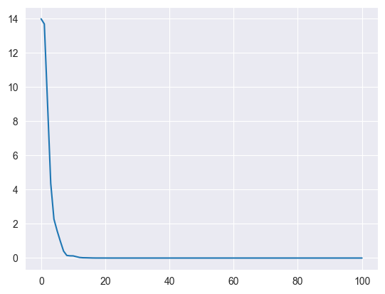

Q6

Derive the partial derivative of the error with respect to a single entry of \(\mathbf{x}^{(k)}\) (without loss of generality, we will say \(x^{(k)}_1\)). Work in the expanded form as in the equation above, writing your answer in the markdown cell below.

Hint: You may find it helpful to refer to the latex equation cheatsheet on the course website. You may show intermediate steps here or as handwritten work as a separate file in the repository. The final answer should be filled in here.

Answer

\[\frac{\partial e^{(k)}}{\partial x^{(k)}_1}= \frac{\partial}{\partial x^{(k)}_1} \sum_{i=1}^n \left(\sum_{j=1}^n A_{ij}x^{(k)}_j - b_i\right)^2\]

Apply sum and chain rules \[= 2\sum_{i=1}^n \left(\sum_{j=1}^n A_{ij}x^{(k)}_j - b_i\right) \frac{\partial}{\partial x^{(k)}_1}\left(\sum_{j=1}^n A_{ij}x^{(k)}_j - b_i\right)\] Apply sum rule noting that \(\frac{\partial}{\partial x^{(k)}_1}A_{ij}x_{j} = 0\) for \(j\neq 1\).

\[=2\sum_{i=1}^n \left(\sum_{j=1}^n A_{ij}x^{(k)}_j - b_i\right) A_{i1}\]

In practice, we will likely want to compute the derivative with respect to all entries of \(\mathbf{x}\): \[\frac{\partial e^{(k)}}{\partial \mathbf{x}^{(k)}} = \begin{bmatrix} \frac{\partial e^{(k)}}{\partial x^{(k)}_1} \\ \vdots \\ \frac{\partial e^{(k)}}{\partial x^{(k)}_n} \end{bmatrix}\]

Q7

Using the formula you just derived, write the formula for the vector of all partial derivatives in the compact matrix/vector notation (e.g. \(A\mathbf{x}=\mathbf{b}\)).

Answer

\(\sum_{j=1}^n A_{ij}x^{(k)}_j\) of the \(i^{th}\) entry of the matrix-vector product \(\mathbf{A}\mathbf{x}^{(k)}\) \[=2\sum_{i=1}^n \left( (\mathbf{A}\mathbf{x}^{(k)})_i - b_i\right) A_{i1}\]

Similarly subtracting \(b_i\) corresponds to vector subtraction with the vector \(\mathbf{b}\) \[=2\sum_{i=1}^n \left( \mathbf{A}\mathbf{x}^{(k)} - \mathbf{b}\right)_i A_{i1}\]

Finally we’re left with the equivalent of a dot product for entry 1!

\[\frac{\partial e^{(k)}}{\partial x_1^{(k)}}= 2 \left( \mathbf{A}\mathbf{x}^{(k)} - \mathbf{b}\right)^T \mathbf{A}_{1}\]

If we remove the index into \(\mathbf{A}\), we get an expression for the gradient! \[\frac{\partial e^{(k)}}{\partial \mathbf{x}^{(k)}}= 2 \left( \mathbf{A}\mathbf{x}^{(k)} - \mathbf{b}\right)^T \mathbf{A}\]

Q8

Do you notice any relationship between this result and the Richardson iteration algorithm above? (1-2 sentences) We will discuss this more in class!

Answer

We see that this gradient is almost equivalent to the update we made in our Richardson iteration, but scaled by \(-2\mathbf{A}\)!

Part 2: Working with batches of vectors

Recall that a vector can also be seen as either an \(n \times 1\) matrix (column vector) or a \(1 \times n\) matrix (row vector).

\[\text{Column vector: } \mathbf{x} = \begin{bmatrix} x_1 \\ x_2 \\ x_3 \end{bmatrix}, \quad \text{Row vector: } \mathbf{x}^T = \begin{bmatrix} x_1 & x_2 & x_3 \end{bmatrix}\]

Note that we use the same notation for both as they refer to the same concept (a vector). The difference becomes relevant when we consider matrix-vector multiplication. We can write matrix-vector multiplication in two ways: \[\text{Matrix-vector: }A\mathbf{x} = \mathbf{b}, \quad \text{Vector-matrix: }\mathbf{x}^TA^T= \mathbf{b}^T\] In matrix-vector multiplication we treat \(\textbf{x}\) as a column vector (\(n \times 1\) matrix), while in vector-matrix multiplication we treat it as a row vector (\(n \times 1\) matrix). Transposing \(A\) for left multiplication ensures that the two forms give the same answer.

Q9

Using the previously defined \(\mathbf{x}\), create an explicit column vector and row vector. Then using the previously defined \(A\), verify that the matrix-vector and vector-matrix multiplications shown above do produce the same resultant vector \(\mathbf{b}\).

Hint: Recall that np.dot is also used for matrix-matrix multiplication. The values of \(\mathbf{x}\) and \(A\) are: \[\mathbf{x} = \begin{bmatrix} 1 \\ -2 \\ 1 \end{bmatrix}, \quad A = \begin{bmatrix} 4 & -3 & 2 \\ 6 & 5 & 1 \\ -4 & -1 & 2 \end{bmatrix}\]

Answer

x_col = x[:, None] # Add new diminsion 1
x_row = x[None, :] # Add new dimension 0
print(np.dot(A, x_col), np.dot(x_row, A.T))

[[ 2.]
 [-1.]
 [ 3.]] [[ 2. -1.  3.]]

The distinction between row and column vectors also affects the behaivior of other operations on np.array objects, particularly through the concept of broadcasting.

Q10

Consider a \(3 \times 3\) matrix of all ones as defined in code below, along with the 1-d vector \(\mathbf{x}\).

ones = np.ones((3, 3))
x = np.array([1, -2, 1])
ones

array([[1., 1., 1.],
       [1., 1., 1.],
       [1., 1., 1.]])

Complete the line of code below such that the result of the operation is:

\[\begin{bmatrix} 1 & -2 & 1 \\ 1 & -2 & 1 \\ 1 & -2 & 1 \end{bmatrix}\]

Hint: You should replace SHAPE with an appropriate shape for broadcasting and OPERATION with an appropriate operation (e.g. +, -, *, /)

Answer

result = ones * x.reshape((1, -1))
print(result)

[[ 1. -2.  1.]
 [ 1. -2.  1.]
 [ 1. -2.  1.]]

Throughout this course we will typically use row vectors and vector-matrix multiplication, as this is more conventional in neural-network literature. The concept of row and column vectors becomes handy when transforming collections of vectors.

Recall that a matrix can be seen as a collection of vectors. In numpy we can create a matrix from a list of (1- dimensional) vectors using the np.stack function. This function assumes that the vectors are row vectors creating the matrix as follows: \[\begin{bmatrix} 3 & 1 & -2 \end{bmatrix},\ \begin{bmatrix} 4 & 5 & 3 \end{bmatrix},\ \begin{bmatrix} -2 & -1 & 5 \end{bmatrix}\quad \overset{\text{np.stack}}{\longrightarrow} \begin{bmatrix} 3 & 1 & -2 \\ 4 & 5 & 3 \\ -2 & -1 & 5 \end{bmatrix} \]

We will call this matrix \(X\) to denote that it is a collection of vectors, rather than a single vector (\(\mathbf{x}\)).

Q11

Create this matrix in numpy using th np.stack function.

Answer

X = np.stack([np.array([3, 1, -2]), np.array([4, 5, 3]), np.array([-2, -1, 5])])
print(X)

[[ 3  1 -2]
 [ 4  5  3]
 [-2 -1  5]]

When taken together as a matrix in this way, we can apply the linear mapping \(A\) to all vectors using matrix-matrix multiplication: \[B=XA^T\]

Let’s put this into practice with a visual example.

Q12

Create a \(20 \times 3\) matrix, circle, in numpy of the following form

\[ \begin{bmatrix} \sin(\theta_1) & \cos(\theta_1) & 1 \\ \sin(\theta_2) & \cos(\theta_2) & 1 \\ \vdots & \vdots & \vdots \\ \sin(\theta_{20}) & \cos(\theta_{20}) & 1 \\ \end{bmatrix}\] Where \(\theta_1...\theta_{20}\) are evenly spaced between \(0\) and \(2\pi\).

Answer

theta = np.linspace(0, 2 * np.pi, 20) # Generates 20 evenly-spaced numbers between 0 and 2π

circle = np.stack([np.sin(theta), np.cos(theta), np.ones_like(theta)]).T

The code we just wrote creates a matrix corresponding to a collection of \(20\) row vectors of length 3. Each vector represents a point on the unit circle where the first entry is the x-coordinate, the second entry is the y-coordinate and the third entry is always \(1\): \[ \begin{bmatrix} x & y & 1 \end{bmatrix}\]

Q13

Plot the set of 20 points in circle using the plt.plot function. Use only the x and y coordinates, ignoring the column of 1s.

Answer

plt.figure(figsize=(4, 4))
plt.xlim(-3, 3)
plt.ylim(-3, 3)

plt.plot(circle[:, 0], circle[:, 1])

Q14

Transform all the vectors in circle with the matrix \(A\) using a single call to np.dot. Then plot the original set of points in black and the transformed points in red using the plt.plot function.

You might also consider why we added the extra column of 1s! We will discuss the answer to that in class. \(A\) is the same matrix from q1.

Answer

transformed_circle = np.dot(circle, A)

plt.figure(figsize=(4, 4))
plt.xlim(-10, 10)
plt.ylim(-10, 10)

plt.plot(circle[:, 0], circle[:, 1], c='k')
plt.plot(transformed_circle[:, 0], transformed_circle[:, 1], c='r')

Q15

Finally, shift all the vectors in transformed_circle by the vector \(\mathbf{b}\) defined below, that is, add \(\mathbf{b}\) to every row of the output matrix. Again plot the original set of points in black and the transformed points in red using the plt.plot function.

Hint: the solution to this question should not involve any loops, instead use broadcasting.

b = np.array([4, 1.2, 0])
transformed_circle = np.dot(circle, A) + b

plt.figure(figsize=(4, 4))
plt.xlim(-10, 10)
plt.ylim(-10, 10)

plt.plot(circle[:, 0], circle[:, 1], c='k')
plt.plot(transformed_circle[:, 0], transformed_circle[:, 1], c='r')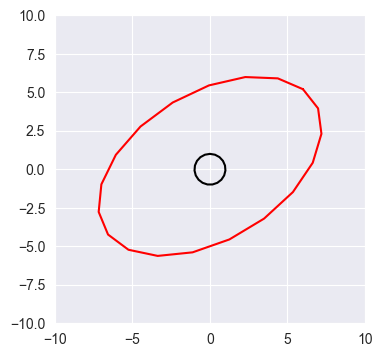

Part 3: Loading and visualizing data

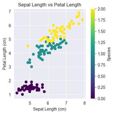
For most of this class we will be working with real-world data. A very well-known dataset in statistics is the Iris flower dataset collected by Edgar Anderson in 1929. The dataset consists of measurments of iris flowers. Each flower has 4 collected measurements: sepal length, sepal width, petal length, petal width, as well as a classification into one of 3 species: Iris setosa, Iris versicolor and Iris virginica. We will return to this dataset in the next homework.

We can load this dataset as Numpy objects using the Scikit-Learn library. Below we’ve extrated 4 relevant arrays: - features: a matrix which has one row per observed flower and one column per measurement. - targets: An array that specifies the species of each flower as a number 0-2. - feature_names: a list of strings with the name of each measurement. - target_names: a list of strings with the name of each species.

In this homework, we will only visualize this dataset, which is typically a good first step in working with a new type of data. We’ll start by just looking at 2 measurements sepal length and petal length, along with the species.

Q16

Based on the Iris dataset loaded below, how many flowers did Edgar Anderson measure?

In other words, how many observations are in this dataset?

Answer

import sklearn.datasets as datasets
dataset = datasets.load_iris()
features = dataset['data']
targets = dataset['target']
feature_names = dataset['feature_names']
target_names = dataset['target_names']

# Answer
num_observations = features.shape[0]
print(num_observations)

150

Fill in the code to create a scatterplot for the Iris dataset below. Plot sepal length on the x-axis and petal length on the y-axis. Set the color to correspond to the species.

# Fill your code here

plt.figure(figsize=(4, 4))
plt.scatter(features[:, 0], features[:, 2], c=targets, cmap='viridis')
plt.xlabel('Sepal Length (cm)')
plt.ylabel('Petal Length (cm)')
plt.title('Sepal Length vs Petal Length')
plt.colorbar(label='Species')